SNT 和 Sholl 分析 基于 publications。请在您自己的研究中cite！

此页面最后一次修订为 version 5.0.0.
请直接通过本页第 editing 帮助我们保持最新文档，以填补任何文档空白。如果您需要帮助，请执行reach out！

用于直接分析分割图像和追踪形态的自动化 Sholl。具有基于曲线拟合的强大量化功能。也可以对其他软件获得的配置文件进行分析。

＃ 介绍 The Sholl technique[^2] is used to describe neuronal arbors. SNT features a collection of tools that perform Sholl on reconstructed morphologies, or directly on 2D/3D images of isolated neurons (bypassing the need for reconstruction). The procedure is based upon how Sholl analysis is done by hand: Algorithms define a series of concentric shells (circles or spheroids) around a focal point of a neuronal arbor and count how many times the arbor intersects sampling shells. The major advantages of these tools over other implementations are:

• 图像和重建都可以分析
• 直接分析图像时，不需要预先跟踪乔木
• Curve fitting与多个methods相结合，自动从采样数据中检索quantitative descriptors，从而可以在乔木之间进行直接统计比较
• 允许围绕用户定义的焦点进行Continuous and repeated sampling
• Angular、length-based 和 intensity-based 配置文件
• 广泛的定量分析选项
• Batch processing是可能的

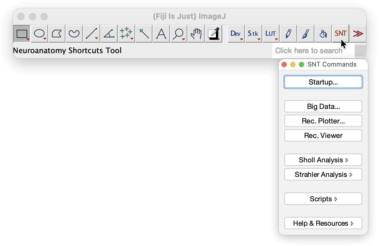
在 installing SNT 之后，可以通过 Plugins › Neuroanatomy › Neuroanatomy Shortcut Window（ImageJ 工具栏中的 SNT 图标）或从 SNT 的 tracing interface 访问 Sholl 命令。

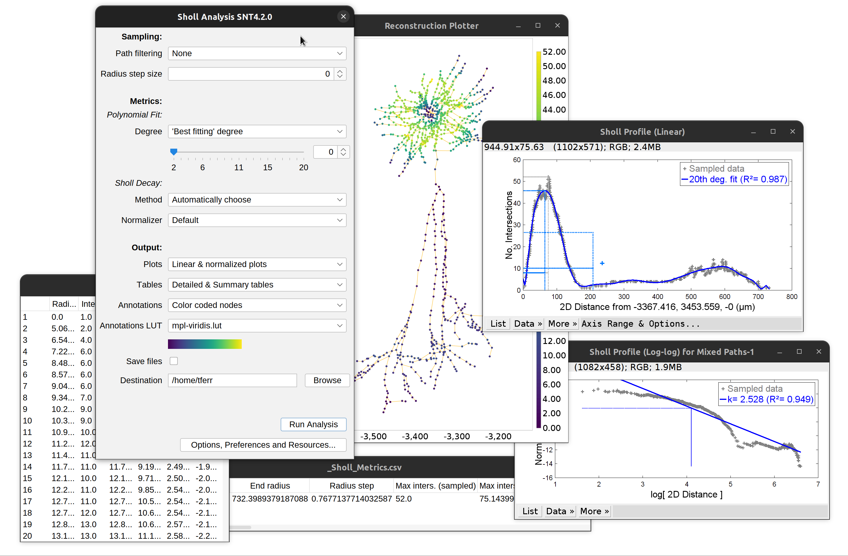Overview of outputs: Linear and log-log profile (Sholl decay calculation), detailed and summary tables. ‘Traditional’ plots are obtained by disabling curve-fitting altogether

Skeletonized hippocampal CA1 cell¹ in which apical and basal dendrites have been analyzed separately and color coded according to their Sholl profile. Warmer hues indicate higher number of Intersections (N). Critical radius (r_c) 和 Mean value (N_av) are indicated.

Linear plot for the same CA1 cell¹. Using the soma as center, image was sampled twice using hemishells in order to segregate apical from basal dendrites. For clarity, distances for basal branches were assigned negative values and arbor overlaid (in green) over the profile.

Combine Sholl Profiles… aggregates individual profiles into a single plot, obtaining the average profile for groups of cells [use case]

Statistics for groups of cells [use case]

Sampled data can be fitted to polynomials of varying degree (animation created using BAR)

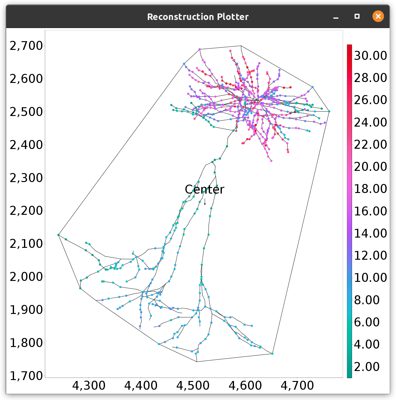Scripting allows for arbitrary focal points, in this case the centroid of the neuron’s convex hull (Convex Hull as Center template script)

Angular Sholl and Angle-based metrics

Intersection points and sampling shells can be retrieved as annotation ROIs

Using Sholl to measure the distribution of image objects (Sholl Rasterize Shells template script) [use case]

Not only neurons: Integrated-density profiles can be used to obtain radial maps of fluorescent markers.

配置文件类型

基于长度的配置文件

自从 SNTv5 以来，除了传统的 No. 之外，还可以获得 **长度配置文件。交叉路口**计数。这两种策略通常（高度）相关但不相同：_交叉计数_总结乔木穿过每个采样壳的频率（交叉频率）。 _长度_总结了每个外壳内有多少电缆。 For direct parsing of images, groups of foreground pixels are first identified along each sampling shell:

• Groups are defined as 8‑connected components in 2D and 26‑connected in 3D
• The No. of Intersections at a shell is the number of identified groups
• The Intersected length at a shell is the sum of path lengths of all groups within that shell. Note that lengths can be affected by the apparent thickness of processes. Consider skeletonizing before analysis to reduce thickness bias

For traced morphologies, each segment (straight line between consecutive nodes) is tested against each sampling shell:

• If a segment intersects a shell, the segment is clipped to the shell and its arc length inside the shell is accumulated
• Intersections at a shell correspond to the number of connected arbor components that cross the shell (based on the tracing graph topology, not pixel connectivity)
• Length at a shell corresponds to the sum of Euclidean lengths of all clipped segment pieces inside that shell. Note that node radii are not considered for length calculations 注意：
• 从概念上讲，长度需要非零的 radius step size。如果选择连续采样（步长 = 0），程序将在内部回退到_最小_分离：解析图像时体素维度的几何平均值，或解析重建时结构的中值节点间距离
• 报告的长度采用校准单位（例如 µm）

基于强度的配置文件

When parsing images directly it is possible to obtain integrated density plots. In this case rather than reporting on No. of intersections or intersected lengths, these profiles report on normalized integrated density. Normalized integrated density is the sum of all voxel intensities along the sampling shell normalized to the perimeter/surface of the shell. These type of profiles can also include cumulative distributions plots and are useful to quantify the distribution of organelles and other structures in cells (including non-neuronal cell types), e.g., as in:

• 细胞核内 FISH 斑点的分布：doi:10.1371/journal.pgen.1010451
  • 线粒体的分布：doi:10.1016/j.celrep.2016.09.004

基于体积的配置文件

When parsing tracings, it is possible to profile intersected arbor volume. This is achieved by clipping each traced segment to the sampling shell and summing the volumes of the resulting truncated-cone (frustum) pieces.

图像直接分析

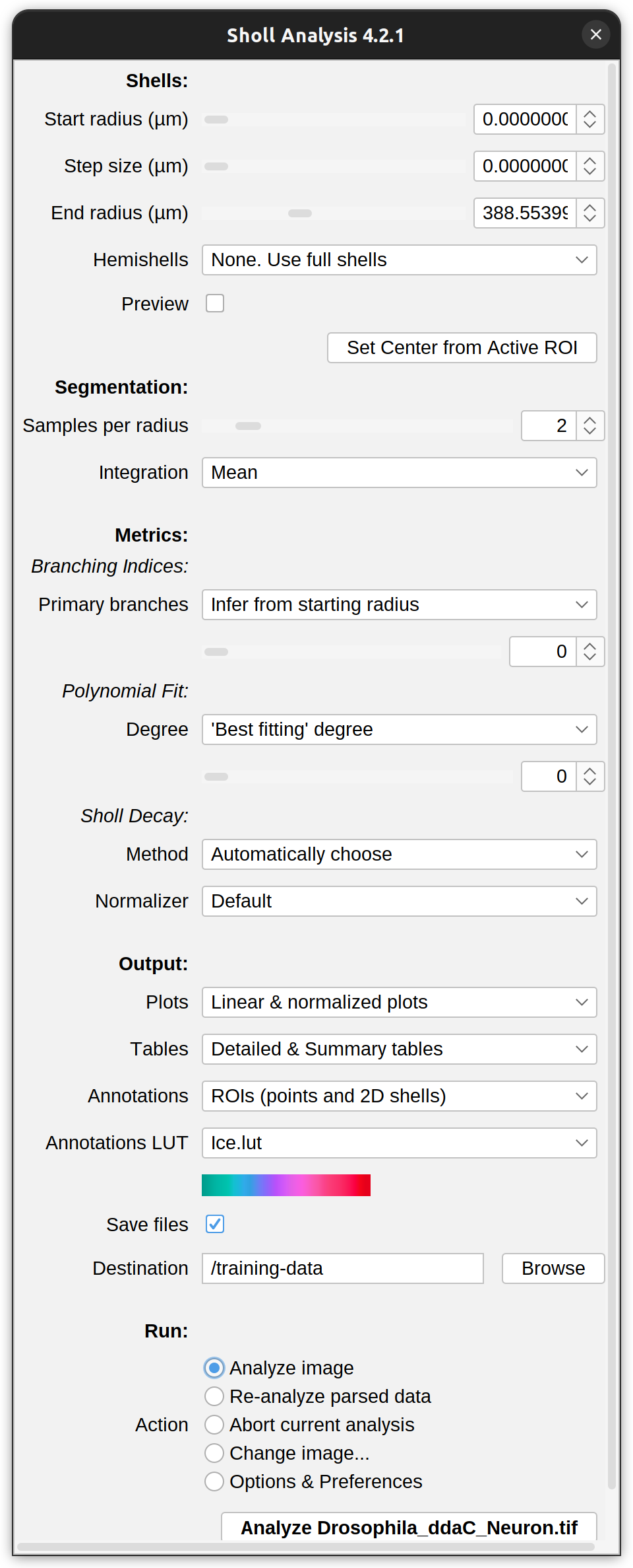在此模式（位图分析）下，插件需要包含单个神经元的 binary image or a segmented grayscale image（2D 或 3D）。

1. 使用Image › Adjust › Threshold…（快捷键：⇧ Shift + T）分割神经元轴。使用多通道图像时，您必须使用Image › Color › Channels Tool…（⇧ Shift + Z）将显示模式设置为灰度，因为显示为复合的图像无法进行阈值处理。
2. Visually inspect 图像中的两个阈值阶段，以确保解析 arbor 而不是 background。
3. 使用有效的startup ROI定义分析中心。
4. 运行Analysis › Sholl › Sholl Analysis…，调整对话框提示中的默认Parameters。
5. 有问题吗？阅读第FAQs。

启动投资回报率

可以使用以下三种可能性之一指定分析中心：

1. 直线：使用直线工具从心轴的焦点到其最远点的直线。使用线选择的优点有两个：1) 自动设置分析中心和Ending radius，2) 水平/垂直线（通过在使用直线选择工具时按住⇧ Shift创建）可用于图像的restrict analysis to sub-regions。

2. 单点：使用点选择工具标记心轴焦点的单点。通过单点选择，仅定义分析中心。因此，此选项适用于具有未定义 Ending radius 的不同尺寸的batch processing 图像。

3. 多点选择：多点选择（多点计数器），其中第一个点标记分析中心，而其余点标记（计数）计算ramification indices）所需的主要分支数量。适用于inference from starting radius无效的情况。

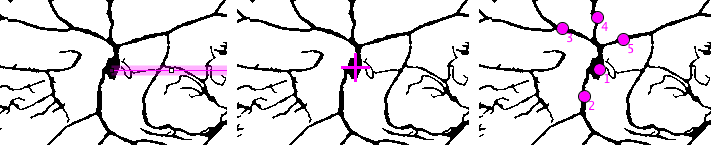
直接分析图像时插件预期的三种类型的 ROI。 左：定义分析中心（焦点）、半球限制和结束半径的线。 中间：单点定义分析中心。 右：多点选择，其中第一个点定义焦点，而其余点（2至5）用作初级神经突的计数器。

参见。分割

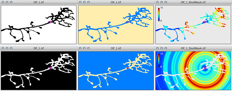
目视确认对分割图像的哪个相位进行采样非常重要，特别是在使用黑白（二进制）查找表时。为此，您可以选择“阈值”小部件中的_红色_查找表 (Image › Adjust › Threshold… ⇧ Shift + T) 以突出显示背景像素中的前景，以验证您正在测量神经元过程，而不是它们之间的间隙空间。下面是一个使用果蝇嗅觉神经元 demo dataset 轴突轴的示例：

分割图像 （黑/白LUT） 分割图像 （黄/蓝查找表） 交叉点蒙版 （喷射查找表）

顶行：图像正确分割：对 Arbor 进行采样。底行：异常分割（倒像）：对背景进行采样。 Note the reversal of output and how the 交叉点掩模不再装饰轴突，而是装饰轴突之间的间隙。相位反转的后果是双重的：1）程序过采样（参见左上角的色调斜坡）交叉点蒙版) 和 2) 程序检测图像边缘引起的伪影（参见掩模的右上角和右下角，在这些位置没有真实轴突的情况下对交叉点进行采样）。另请注意，初始黑白图像将看起来一样 under an inverted lookup table (Image › Lookup Tables › Invert LUT).

追踪细胞分析

在此模式下，插件分析重建的乔木（在 SNT 或 elsewhere 中追踪），这对于不允许单细胞分辨率或正确分割的染色特别相关。这个分析有几个切入点，即：

• SNT的主界面：提供更多用于定义分析中心、标记分支限制等的选项，但不适合批处理。

• 通过 Plugins › Neuroanatomy › Neuroanatomy Shortcut Window（ImageJ 工具栏中的 SNT 图标）访问 Sholl Analysis（轨迹） 命令：适用于不需要查看轨迹的情况，或需要 batch processing 时

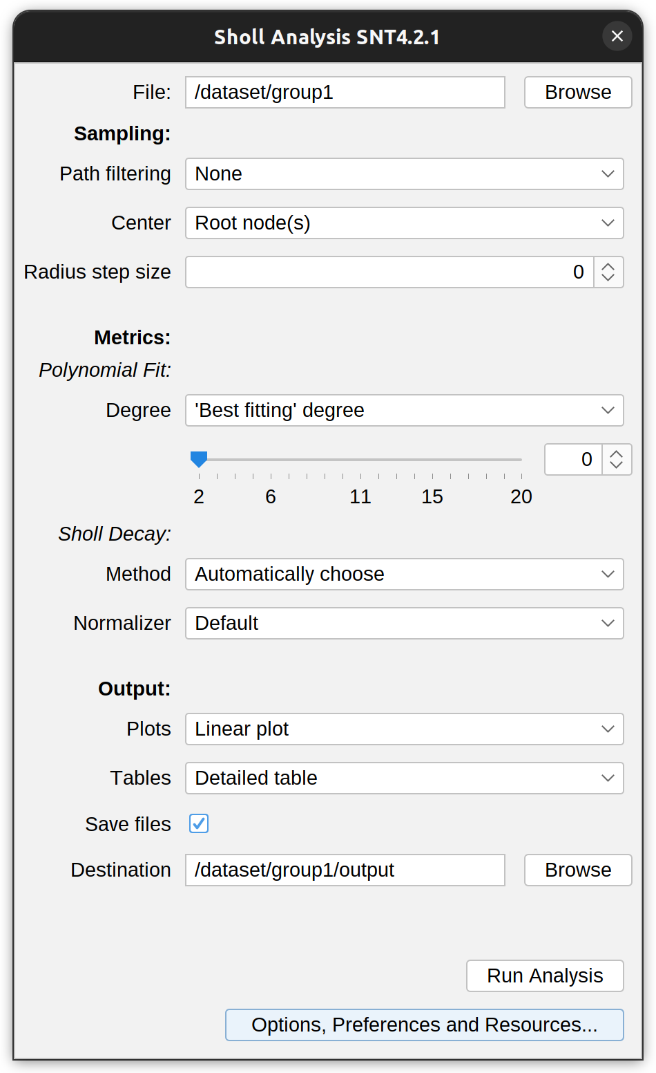
要分析细胞而无需初始化 SNT 的跟踪接口，请运行 Sholl Analysis (Tracings)… 并指定：

• 文件 要解析的 tracing file（swc、.ndf、.json 或 .traces 扩展名）

• 路径过滤 分析是否应限制在特定路径，例如标记为（axon、dendrite、soma 等）的路径。请注意，如果您的追踪未标记，您可以在 SNT 中进行标记

• 中心 分析中心，定义为：
  • Root nodes These correspond to the starting nodes of primary (root) paths. If multiple primary paths exist, center becomes the centroid (mid-point) of their starting nodes
  • Soma node(s) These correspond to nodes tagged as “soma”. If Ignore connectivity is chosen, the centroid of all soma-tagged nodes is used, even if such nodes are not at the root of the structure. If Primary paths only is chosen only root nodes tagged as “soma” are considered

• 指标和输出 这些在 Curve fitting、Choice of Methods 和 Output options 中进行了描述。

• 高级选项 这些选项包含在_选项、首选项和资源_对话框中，包括：

  • 跳过体细胞片段 如果主要路径从距离体细胞“很远”的地方开始，则此选项允许忽略体细胞和神经突之间的片段。请注意，仅当正在分析的乔木植根于标记为“Soma”的单节点时才考虑此选项

  • 包括零计数 与 0 个交叉点相关的条目是否应包含在详细表格、绘图等中。

现有配置文件分析

This option allows curve fitting to be applied to previously sampled profiles and is achieved via scripting. It requires only a tab or comma delimited text file (.csv, .txt) listing a sampled Sholl profile. Have a look at the Sholl Extensive Stats Demo template script for more details.

参数

某些参数特定于用作输入的数据类型，无论是分段图像还是重建（跟踪）。分析图像时，输入值会考虑图像的比例信息（可以使用Analyze › Set Scale…或Image › Properties…（⇧ Shift + P）设置）、图像类型（2D或3D）及其active ROI。

为了清楚起见，与图像直接解析相关的设置用 标记，与重建（追踪）相关的设置用 标记。

贝壳

配置文件类型

Whether the profile should report traditional No. of intersections counts or intersected lengths

起始半径

The radius of the smallest sampling circle/sphere, i.e., the first distance to be sampled. ####步长 The sampling interval between radii of consecutive sampling circles/spheres. This value may be set to zero for continuous (1-voxel increment) measurements. For stacks with anisotropic voxel size, setting Radius step size to zero, sets the step length to the dimension of the matching isotropic voxel, i.e., the geometric mean of voxel dimensions: For 3D images, the cube root of the product of the voxel dimensions; For 2D images: the square root of the product of the pixel dimensions.

结束半径

The radius of the largest (last) sampling circle/sphere. It is automatically calculated if a line ROI is used. Note that the specified distance may not be actually sampled, if Radius step size is not a divisor of Ending radius-Starting radius. In this case, the program will choose the largest possible distance smaller than the specified value. You can clear Ending radius or set it to NaN (“Not a Number”) to sample the entire image. This is particularly useful when batch processing images with different dimensions.

半壳

This option can be used to limit the analysis to sub-compartments of the arbor. This option instructs the algorithm to measure intersections at sites equidistant from the center that have y-coordinates above/below the drawn line or x-coordinates to the left/right of the center. ＃＃＃＃ 预览 Previews sampling shells on the image being analyzed. Note that with 3D images, the previewed 2D circumferences do not reflect the actual 3D spheres used by the algorithm.

设置活动 ROI 的中心

Updates the center position by reading the centroid of the active ROI.

降噪

每个半径的样本 （仅限 2D 图像）

Defines the number of measurements to be performed at each sampling circumference. These measurements are then combined into a single value according to the chosen integration method. This strategy, a break from previous approaches, increases the accuracy of non-continuous profiles by diluting out the effect of processes extending tangent to the sampling circumference. 从视觉上看，此选项可以想象为采样圆周的“厚度”：例如，对于 100 个像素的半径和 3 个每个半径的采样数，最终的交叉点数量将整合在距离 99、100 和 101 处采样的测量值。请注意，增加采样数超过半径步长的长度（以像素为单位）是没有意义的。因此，此选项仅限于严格（且任意）最多 10 个样本。

示例集成 （仅限 2D 图像）

The measure of central tendency used to combine intersection counts when multiple Samples per radius are used. Options are Mean (the default), Median or Mode.

忽略孤立的体素 （仅限 3D 图像）

Accessed through the Options & Preferences dialog. If checked, single (6-connected) isolated voxels intersecting the surface of sampling spheres are not taken into account, which may allow for smoother profiles on noisy image stacks. However, it should be noted that connectivity in the stack volume may not reflect connectivity on the surface of a digitized sphere. Indeed, in certain contexts, it is possible (though unlikely) to obtain higher intersection counts when this filtering option is active. 请记住，这只是一个细化功能，您不应期望它能够减轻由于不良分割而产生的主要工件。

并行线程数量 （仅限 3D 图像）

Accessed through the Options & Preferences dialog. Sets the max. no. of parallel threads to be used when parsing 3D stacks. Note that this options also sets the no. of threads used by ImageJ and SNT for other multithreaded tasks. Set it to 0 to use all of the available processors on your computer.

主分支数量

The number of primary branches (i.e., those originating directly from cell soma when the center of analysis is the perikaryon) to be used in the calculation of Schoenen ramification indices. This option is only relevant when computing branching indices. Set it to zero to disable calculations of ramification indices. Choices include:

• 从起始半径推断 如果选中，主分支数量 是根据 Starting radius 处的交叉点计数推断的。
• 从多点 ROI 推断 如果多点 ROI 为 detected at startup，则使用多点计数。

多项式拟合

Specifies the degree of the polynomial to be fitted to the Linear profile². While the polynomial of best approximation, or “best fit”, should be empirically determined for each analyzed cell type, it is possible to ask the plugin to predict the order of the fitting polynomial (or at least try) using the choice Best fitting degree. In this case, the plugin will loop through all the available choices of polynomials, perform each fit in the background and choose the one with the highest coefficient of determination. 对多项式拟合的详细控制由 Options & Preferences 提示中的选项控制，即：

• 最小。次数 计算“最佳拟合”多项式时要考虑的最低阶次
• 最大。度数 计算“最佳拟合”多项式时要考虑的最高阶数（可能不支持 40 以上的度数）
• R 平方截止 用于丢弃“不适当拟合”的确定系数 (R²) 截止。仅考虑与大于此值的 R^2 相关的拟合
• K-S 验证 如果两个样本 Kolmogorov-Smirnov 检验拒绝拟合值和分析值是从相同概率分布中抽取的样本的零假设 (p<0.05)，是否应放弃拟合

标准化

Options for computing metrics based on normalized (Semi-log or Log-log profiles), including Sholl decay.

• 方法 指定方法的类型。当您无法预测哪种类型的标准化配置文件最能描述数据集时，请选择“自动选择”。如果选择，插件将使用 Determination ratio 来确定 Semi-log 或 Log-log 方法中哪种更合适。

• 归一化器 用于线性范数、半对数和对数-对数配置文件归一化的采样外壳属性。默认为面积（2D 图像）/体积（3D 图像）。这是described below。

输出选项

Defines which kind of annotations should be output, including:

• 绘图 要输出的绘图类型。除了 Linear and Normalized profiles 之外，还可以获得 polar plots 以及 intensity-based 配置文件的累积分布图。

• Tables 定义应输出哪种类型的表，包括_Detailed_ 和_Summary_ 表。

• Annotations 定义应输出哪种类型的注释，包括：

  • LUT 用于注释的查找表 (LUT)。

  • ROI 允许将两组 ROI 添加到图像叠加中：1) 与采样距离匹配的同心壳（圆形 ROI 或使用半圆时的复合 ROI）； 2) 外壳和前景像素簇之间交叉点处的多点 ROI。请注意，这些蒙版的所见即所得版本（RGB 图像）可以通过按 ⇧ Shift + F (Image › Overlay › Flatten) 或运行 Analyze › Tools › Calibration Bar… 来获得。 NB:

    • ROIs are not created when outputting integrated density
    • Versions prior to SNTv5 placed intersection points at edges of detected clusters of foreground pixels, not their centroid

• 掩模 生成分析图像的 16/32 位最大强度投影，其中根据其 Sholl 轮廓绘制测量的乔木。数据类型（Raw，即采样或Fitted）显示在图像字幕中

• 保存文件 如果选中，输出将保存到指定目录。文件以图像文件名命名。

• 显示配件详细信息 - 选择此选项可将单纯形配件的所有参数打印到日志窗口。即使未选择此选项，coefficient of determination（R²，拟合优度的度量）也始终存储在 Sholl 结果 表中

肖尔图

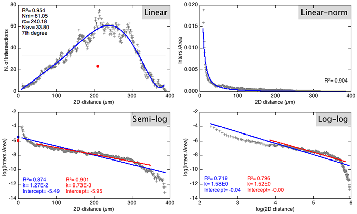
ddaC demo dataset的线性、线性范数、半对数 和 对数-对数 配置文件。大部分检索到的 metrics 都会被插件自动突出显示。 线性轮廓：Mean value（水平网格线）和Centroid（彩色标记）。对数剖面：Sholl regression coefficient（也称为 Sholl 衰减）可以使用全范围数据（蓝线）或百分位数 10-90 内的数据（红线）通过线性回归来检索。对于这种特定的细胞类型，与对数对数方法相比，半对数方法更加informative。 其他类型的图请参见Angular Sholl。

N对于 2D 图像，N与半径 r 的圆周相交的像素簇（8 个相连）的数量
对于 3D 图像，Number of clusters of voxels (26-connected) intersecting the surface of the sphere of radius r

r距分析中心的距离（radius of Sholl circle/sphere)

日志 Natural logarithm, the logarithm to the base e

S The property of the sampling shell to be used in the normalization of Linear-norm, Semi-log, and Log-log profiles. 对于 2D 图像，采样周长 (2πr) 的 周长 或相应圆的 面积 (πr²) 对于 3D 图像，采样球体的表面 (4πr²) 或其各自的体积 (4/3πr³) Annulus/Spherical shell normalization is also available when performing non-continuous sampling. In this case, the normalization is performed against the area/volume between circumferences/spheres at r ± Radius step size/2

角壳

Angular Sholl（半径 × 角度，也称为 Polar Sholl）生成极地热图，以揭示 Sholl 剖面中的方向偏差以及此类偏差如何随距离变化。 Angular Sholl 将 Sholl 交点的位置（即“Sholl 点”）分布在有角度的扇区上。总结_No。每个半径上的交集_（或_相交长度_）会产生一个角度分布，用于计算angle-based metrics。

简而言之，Angular Sholl 中检测首选方向的算法的工作原理如下：

1.“指南针直方图”：想象神经元周围的空间像披萨一样被分成相等的切片（例如，每 10°）。对于每个切片，程序会累加每个方向有多少心轴点 - 交叉数量（“交叉点”）或交叉电缆的数量（“长度”）

1. 平滑：每个切片与其两个相邻切片进行平均，以减少噪声引起的抖动

2. 识别突出切片（“峰值”）：程序使用局部突出度（与两个相邻切片的平均值的差异）来测量切片相对于其直接相邻切片的“高”程度。只有具有强烈突出性的较高切片才被视为真正的峰值

3. 曲线拟合：如果仅识别出一个峰，则将分布角拟合为von Mises distribution。如 Root Angle Analysis 中详述，这是对角度/方向建模的正态分布的圆形模拟

4. 此过程结束后，将获得定向“峰值”列表：每个峰值都有一个角度（以度为单位）和一个强度（该切片的高度）

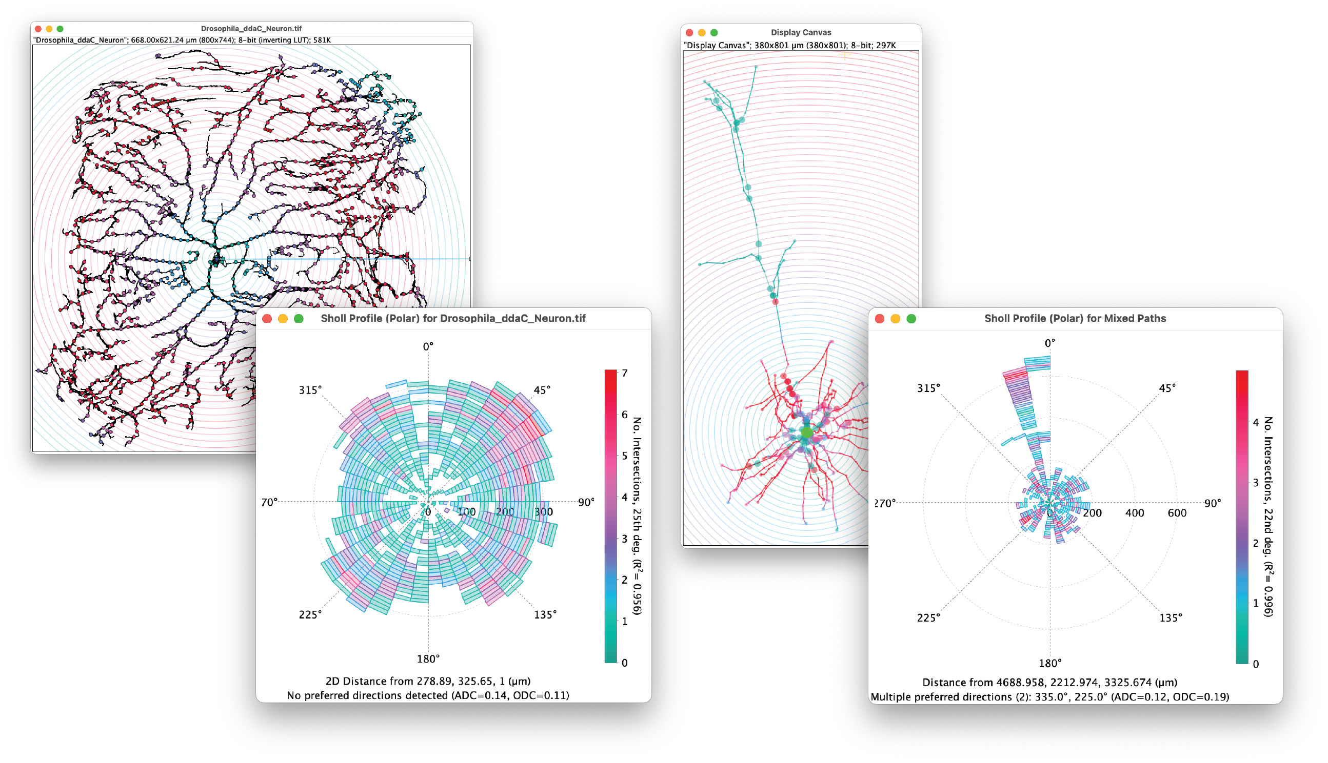角（极）剖面示例。左：ddaC 演示数据集的空间填充树突，具有同质 angle distribution。右：锥体神经元（MouseLight 树突演示数据集）。基底树突与均匀的角度分布相关，但顶端树突具有很强的directional bias。在这两个原因中，都使用了 10° 的 bin 宽度。可以为length-based profiles和fitted data获得此类数据。

指标

心轴的形态描述符和其他属性被打印到测量表中。可以使用分析提示中“更多选项”对话框中的_详细指标_复选框来自定​​义输出。

基于采样数据的指标

• 分支指数 (BI) 总结由 Garcia-Segura 和 Perez-Marquez³ 定义的神经突树枝化的指数。请注意，该指数广泛受半径步长的影响。在不同采样的细胞之间比较该指标将是无意义的，如demonstrated here。报告此指标时，应始终包含步长（例如，BI_10μm=20）。

• 质心半径 线性轮廓的centroid（即几何中心或重心）的横坐标。它是N 与距离 图上的highlighted。

• 质心值 线性轮廓的centroid（即几何中心或重心）的纵坐标。它是N 与距离 图上的highlighted。

• 封闭半径 最后一个（即最宽的）相交半径与Enclosing radius cutoff指定的交叉点数量相关联。对于截止值 1（默认值），封闭半径 是相交半径 中最宽的一个。它反映了乔木的Feret length。

• 峰度 采样数据的kurtosis，它量化分布的形状是否与高斯分布匹配，假​​设高斯分布的峰度为 0。比高斯分布更尖峰的分布具有正峰度，而负值表示分布更平坦。另见Kurtosis (fitted data)

• 最高交叉点数量 (最大交叉点) 采样交叉点的最大值，即线性 [N vs 距离] 轮廓中的最大值，反映了乔木中进程/分支的最高数量。另请参见Critical value。

• 相交半径 与心轴相交至少一次的采样半径的数量。

• 相交平均值（平均相交） 相交总和除以相交半径。另请参阅Mean value、FAQ

• 交叉点中位数 (Median Inters.) 采样交叉点的中值。

• 交叉点最高计数的半径（最大间隔半径） 交叉点最高计数发生的距离，反映了最高分支密度的位置。请注意，如果相同的最大值出现多次，则仅考虑第一个距离。另见Critical radius

• Schoenen 分枝指数（分枝指数（采样）） 分枝的度量⁴：最大间隔 与 primary branches 数量之间的比率。仅当 primary branches 有效且不为零时才计算。另请参见Ramification index (fit)

• 偏度 采样数据的skewness，表明分布围绕其平均值的对称程度。正值表示不对称分布，右侧有较长的尾部。负值表示左侧尾部较长的数据。流行的经验法则认为，如果偏度大于 1.0（或小于 -1.0），则分布可能被认为非常不对称。另请参阅Skewness (fitted data)

• 交集总和 (Sum inters.) 所有交集总和。
  
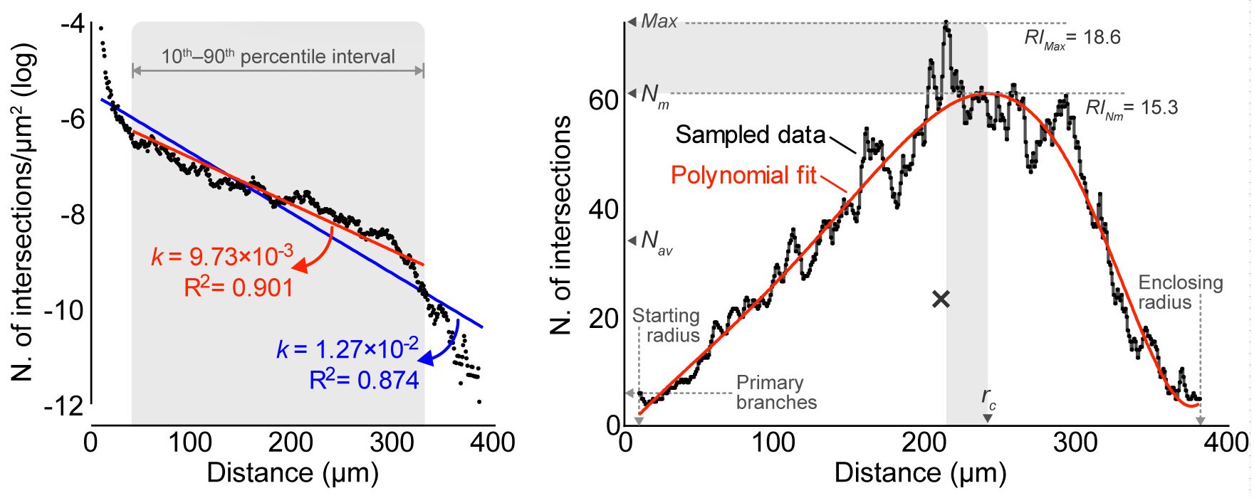  Overview of Sholl metrics) based on curve fitting including the Sholl regression coefficient (k), Critical value (Nm), Critical radius (rc) and Mean value (Nav). Differences between sampled and fitted maxima are shaded in gray. The centroid of the sampled profile is marked (×). Schoenen ramification index (RI) is the ratio between number of branches at the maximum and the number of primary branches, using either sampled data or the fitted Nm. (Ferreira T, et al., 2014, supplementary booklet)
  
  

  基于拟合数据的指标

• 支化指数（BI 拟合） 从拟合曲线中获得的 branching index。

• 临界半径 临界值出现的距离。默认情况下，其计算精度为半径步长的 1/1000。缩写：r_c。另请参见Max inters. radius

• 临界值 多项式拟合的局部最大值，即(1)中临界半径处的N。缩写：N_m。另见Max inters.

• 判定比 半对数法的coefficient of determination与对数-对数法的coefficient of determination之比⁵。如果半对数方法相对于对数-对数方法更好，则判定比会大于1。它是插件用来默默预测标准化方法的参数，即most informative。可以通过在“选项和首选项”中选择“调试模式”来监视预测。

• 峰度（峰度（拟合）） Starting radius 和 Ending radius 之间拟合多项式分布的kurtosis。

• 平均值 拟合多项式函数(1)的平均值²，代表乔木占据的整个区域的交点平均值。缩写N_av。在 Sholl 图上，它是 highlighted 作为矩形的高度，该矩形的宽度为封闭半径 - 第一相交半径以及该离散区间上拟合曲线下面积的相同面积。它类似于 Mean inters.，整个乔木采样交叉点的算术平均值（参见Metrics based on sampled data）。默认情况下（参见第 Advanced Usage），它的计算精度为 半径步长 的 1/1000。

• 多项式 R² (Polyn.R^2) (1)中描述的多项式拟合的确定系数。

• 回归截距 (3) 和(4) 中描述的 y 坐标 m。

• 回归 R² (回归 R^2) (3) 和 (4) 中描述的线性回归的确定系数。

• Schoenen 分支指数（分支指数（拟合）） 从拟合轮廓中检索的 Schoenen 分支指数：Critical value 和 Number of primary branches 之间的比率。另见Ramification index (sampled)

• 肖尔回归系数（回归系数） (3)和(4)中描述的线性回归的斜率（乘以-1），即k，分支数量随距分析中心距离的衰减率的度量。 k 值越高反映函数 log(N/S) 的变化越大。为了优化拟合，该插件检索以中值距离为中心的 second linear regression，不包括轮廓边缘的距离。当使用 10^th–90^th百分位数内的数据时，第二次拟合的详细信息也会记录在专用列下的Sholl table上，例如，Sholl 回归系数 [P10-P90]。

• 偏度（偏度（拟合）） Starting radius 和 Ending radius 之间拟合多项式分布的skewness。

基于 Angular Sholl 的指标

• 角度分布相干性 (ADC) Sholl data 角度分布的均匀度。无单位，范围为 [0, 1]，值较高表示 Sholl 数据集中在 preferred direction 周围； 0 表示在所有方向上均匀分布。

• 首选方向 (PD) 当Angle distribution coherence较高时，Sholl data最集中的方向。范围：[0°,360°[. Examples: A space filling neuron is not expected to be associated with a prominent direction (low ADC value). On the other hand, a cell may have more than one preferred direction (e.g., data from dendrites of a pyramidal neuron), as exemplified above。

• 方向分布一致性 (ODC) 这是 Angle distribution coherence 的变体，考虑方向而不是方向。 ODC 可用于区分 180° 对称的形态（例如，具有两个相对簇的神经元乔木），对于这些形态，ADC 可能接近 0

• 首选方向 当Orientation distribution coherence较高时，Sholl data最集中的方向。范围：[0°,180°[

与所有其他 Sholl 相关轮廓类似，可以使用交叉计数和 intersecting lengths，以及多项式拟合数据。默认情况下，极地热图使用 10° 的角度箱宽度。可以在分析提示的“更多选项”对话框中调整此灵敏度。

补充工具

SNT 提供了多种脚本和命令，可促进所有类型的 Sholl 相关分析。您可以通过 Plugins › Neuroanatomy › Neuroanatomy Shortcut Window（ImageJ 工具栏中的 SNT 图标）以及脚本编辑器的 Templates › Neuroanatomy 菜单找到它们。

预处理

本节讨论在分割要通过 Sholl 分析 处理的神经元乔木时应考虑的一些方面。由于“图像分割”（即将图像划分为可分析部分）容易受到噪声和背景荧光的影响，因此不可能推广有效二值化灰度图像的通用例程。这意味着任何试图用二元掩模正确描述原始荧光图像的程序都必须根据各个数据集的特征进行定制。

＃＃ 噪音

可以通过使用处理滤波器来减轻噪声。特别有用的是边缘保留过滤器：

• Tubeness和Frangi，参见SNT的Secondary Layer Wizard
• Rolling Ball或“高帽”过滤器，例如Process › Subtract Background…
• 中值滤波 (2D/3D)，例如 Process › Filters、Plugins › 3D
• Anisotropic Diffusion、Plugins › Process › Anisotropic Diffusion 2D
• Sobel 边缘检测，例如 Process › Find Edges
• Shen-Castan 边缘检测器（BAR插件），BAR › Segmentation
• 频率滤波器，例如，Process › FFT › Bandpass Filter…

照明不均匀

当来自组织深层的信号没有像表面层那样明亮时，共聚焦显微镜中确实会出现通常与wide field microscopy相关的不均匀照明问题。沿 Z 轴的信号衰减将在堆栈上生成阴影梯度，histogram-based segmentation 需要考虑这一点。虽然这些问题在采集过程中可以得到更好的解决（例如，使用激光渐变），但可以使用直方图归一化技术来减轻这种影响。例如。：

• Tubeness和Frangi，参见SNT的Secondary Layer Wizard
• Bleach Correction、Image › Adjust
• Attenuation correction

细分

当global thresholding methods不能产生令人满意的结果时，可以采用更复杂的segmentation algorithms。示例：

• Machine learning algorithms（语义分割）
• Local Threshold、Image › Adjust
• Robust Automatic Threshold Selection、Plugins › Segmentation
• Level Sets、Plugins › Segmentation
• Morphological Segmentation、Plugins › Segmentation
• Squassh，分割Bregman图像分割（亚细胞形状的分割和量化，MOSAIC ToolSuite，Plugins › Mosaic › Segmentation
• MorphoLibJ
• BAR用于手动管理阈值图像的脚本，BAR › Segmentation

批处理

SNTv5 恢复了可录制宏命令。因此，最简单/最快的自动化分析方法只需要几个步骤： 1.打开ImageJ的宏录制器：Plugins › Macro › Record…

1. 在“神经解剖学快捷方式”窗口中，从 Sholl Analysis › 的_可录制宏_部分选择相关提示 3.照常设置选项
2. 将录制的字符串复制到宏/脚本中。请注意，记录的表情相当大。确保避免复制/粘贴错误。它应该看起来像：

// 注意：查看 Templates>Neuroanatomy> 中的示例脚本，了解更强大的自动化 Sholl 方法。例如，Sholl_Extract_Profile_From_Image_Demo.py 示例了如何使用 API 调用以编程方式解析图像
run("Sholl 分析（来自图像）...", "datamodechoice=Intersections startradius=0.0 Stepsize=10.0 endradius=400.0 hemishellchoice=[无。使用完整外壳] Previewshells=false nspans=1 nspansintchoice=N/A Primarybrancheschoice=[从起始半径推断] Primarybranches=0多项式选择=['最佳拟合'度数]多项式度= 0 归一化方法描述= [自动选择] 归一化描述=默认plotoutputdescription = [线性，归一化和极坐标图] tableoutputdescription = [详细和汇总表]注释描述= [ROI（点和2D壳）] lutchoice = Ice.lut save = true savingir = / Users / ferreirat Analysisaction = [分析图像]“）;

为了获得更全面的功能，脚本编辑器的Templates › Neuroanatomy菜单列出了执行批处理操作的演示脚本。为了完整起见，这里有一个关于如何从头开始编写宏的小教程：

教程：使用 IJ 宏语言批量分析图像

任何宏都必须设置一个中心，或者允许 Sholl Analysis 插件访问标记它的 ROI。人们可以指示 ImageJ 从文本文件中读取预先存在的 ROI 的坐标，在 ROI 管理器中存储线选择列表，或者编写一个基于形态的例程来检测乔木的中心。然而，标记分析中心可能是您需要手动执行的操作。这是一个工作流程：

1. 将所有要处理的 .tif 图像放在一个文件夹中。
2. 在 ImageJ 主窗口中选择点选择工具。对于 3D 图像，请确保“设置堆栈位置”在 Image › Overlay › Overlay Options… 提示中处于活动状态。
3. 打开第一张图像并按⇧ Shift + T激活阈值小部件(Image › Adjust › Threshold…)。
4. 调整阈值水平。按“阈值”小部件的“应用”按钮创建二进制图像。
5. 选择包含分析中心的 z 切片。使用点选择工具单击中心，然后按B（Image › Overlay › Add Selection…的快捷键）。这会将 ROI 点添加到图像叠加层中。按S (File › Save As… › Tiff…) 将图像另存为 .TIFF。
6. 重复最后 2 个步骤，直到标记所有图像，使用 ⇧ Shift + O（File › Open Next 的快捷方式）迭代所有图像。

现在所有图像都已标记，我们可以使用宏记录器 (Plugins › Macros › Record…) 并对其中一张图像运行 Sholl Analysis 以了解如何使用合适的参数调用插件。在本教程中，我们将使用 ImageJ 宏语言。记录器窗口中显示的单行代码将如下所示：

// 记录 Sholl Analysis 版本 3.4.3
run("Sholl 分析（来自图像）...", "datamodechoice=交叉点开始=10 结束=400 radius_step=0 推断拟合线性多项式=[8 次] 半对数归一化器=体积创建保存");

您可能已经注意到，ImageJ 插件由单个小写句子控制，其中参数由空格分隔。输入字段和选择列表显示为关键字=值对，单个关键字的活动复选框。不需要的选项可以省略。这使得编辑代码块变得更容易：

开始= 10；  // 控制起始半径的变量
结束= 200； // 控制结束半径的变量
步骤=2；   // 控制步长的变量

// 运行插件
run("Sholl 分析（从图像）...", "starting="+ start +"ending="+ end +" radius_step="+ step +" 推断线性保存");

Now we just need to assemble a working macro to be pasted in the Process › Batch › Macro… prompt:

// Get the number of ROIs of the image overlay
nROIs = Overlay.size;
// We cannot proceed if no ROI is available (safety check)
if (nROIs==0)
    exit("No ROI was found. Cannot proceed.");
// Select the last ROI of the overlay. Because we have activated the "Set stack positions" option,
// this will automatically activate the Z-slice in which the ROI was created (3D images)
Overlay.activateSelection(nROIs-1);
// We now call the plugin as detailed by the Macro Recorder. We'll set 'Ending radius' to a non-numeric
// value (NaN, "Not a Value") to make sure the maximum length for each individual image is used
run("Sholl Analysis (From Image)...", "datamodechoice=Intersections starting=10 ending=NaN radius_step=0 infer fit linear polynomial=[8th degree] semi-log normalizer=Volume create save do");

当然，您也可以自动化任何前面的步骤。但是，不要忘记确保调用插件时分析中心可用：

// Impose spatial calibration
run("Properties...", "unit=um pixel_width=1.5 pixel_height=1.5 voxel_depth=3.0");
// Subtract background
run("Subtract Background...", "rolling=50 sliding stack");
// Apply a favorite threshold
setAutoThreshold("Huang dark stack");
// >>>> 确保初始点选择仍然可用<<<<
Overlay.activateSelection( Overlay.size - 1 );
// Run the plugin
run("Sholl Analysis (From Image)...", "datamodechoice=Intersections starting=10 ending=NaN radius_step=0 infer fit linear polynomial=[8th degree] semi-log normalizer=Volume create save do");

就是这样。 Use the Macro Recorder to generate the customizations you will need before parsing the entire folder of images with Process › Batch › Macro…

Complex Scripts

More complex scripts will take advantage of SNT’s API. Here are some of scripts from SNT’s Bundled Templates:

常见问题解答

为了清楚起见，与直接解析图像有关的常见问题解答用 标记，与重建（追踪）相关的常见问题解答用 标记。

一般的

1. How do I cite Sholl Analysis?

Sholl Analysis 的权威参考有两个：

• doi:10.1038/nmeth.3125

• doi:10.1038/s41592-021-01105-7

2. Why do I need to threshold the cell?

计算交叉点实际上是一个二进制过程：shell 要么拦截分支，要么不拦截。因此，图像必须分为两个阶段：乔木和背景。

3. In older versions it was not mandatory to adjust threshold values prior to analysis. Why is it now?

图像分割一直是required。在其早期实现中，该程序仅处理二值图像，并使用分析中心的强度来决定如何将对象与背景分离。这种方法非常严格：它假设代表神经元的像素具有相同（恒定！）的强度，而这在其余背景中是找不到的。当程序意识到灰度图像时，必须删除这个“特征”，因为单个强度不能再用于推断应该分析图像的哪些部分。

4. My images do not look that great. How can I treat them prior to analysis?

看看Pre-processing。

5. My bitmap profiles are different from the ones obtained from tracings of the same cells. Why?

分析的质量取决于乔木的分割方式。如果您使用灰度图像，您可能需要优化您的segmentation routines。 另一方面，如果您已经获得了二进制图像，请确保您是interpreting them properly。您还应该确认 Ending radius 不与图像中分析的乔木之外的其他结构相交。 另请参见The 3D profile looks worse than the 2D profile of the Maximum Intensity Projection of the same cell. Why?

6. My version is not the latest after running Help › Update Fiji… Why?

This may happen if you have manually installed/modified core files.. Run the Updater, choose Advanced Mode then View locally modified files under View Options. Locate files from the Neuroanatomy update site. If the Details pane indicates an available update, click on Locally modified under Status/Action and choose Install/Update. The latest release version will be available once you press Apply changes. See Installation FAQs for more details.

7. This documentation is not that useful. How long do I have to wait until it gets improved?

使用页面第top上的编辑此页面选项并随意编辑其内容。不要害羞。 All changes are undoable!

分析

1. The plugin complains about a wrong image type. Why?

该插件不解析 RGB 图像，但会处理任何灰度图像（8/16 位），包括多通道（复合）图像。这是故意的：RGB 图像不灵活，荧光标记细胞的图像通常是非 RGB 图像。如 ImageJ User Guide 中所述，可以使用 Image › Color › Channels Tool… 或 Image › Type 命令转换 RGB 图像。

2. With 3D and 4D images, how do I set the Z-position of the center?

分析中心的 Z 位置（深度）是堆栈的活动 Z 切片。对于多通道（复合）图像，活动通道还定义 C 位置。两者均报告在Sholl 结果表中。

3. Why so many parameters?

该插件专为分析各种乔木而设计，并且不偏向任何特定细胞类型。确保这种广泛适用性的唯一方法是让用户完全控制插件用于分析采样数据的数学技术。

结果

1. How can I save/edit the Sholl Results table?

Use Fiji’s File › Export › Table… command or SNT’s File › Save Tables and Analysis Plots… (details), or right-click on the table and choose Save As…

2. What is the Sholl mask?

Sholl 掩模 (see example of CA1 cell) 只是一个示例：所分析细胞的最大强度投影，其中intersection counts 用作像素强度。如第 Output Options 中所述，可以修改其 LUT，并使用 ImageJ 默认命令校准强度。如前所述，它还可用于目视检查 segmentation artifacts。

3. The 3D profile looks worse than the 2D profile of the Maximum Intensity Projection of the same cell. Why?

各向异性体素大小将对step size产生强烈影响。另一方面，根据options chosen，2D 和 3D 图像可以进行不同的采样。 如果Image › Properties…（⇧ Shift + P）报告适当的空间校准，请检查Noise Reduction参数。 Analysis › Sholl Bitmap vs Tracing Comparison template script 可用于比较不同输入的 Sholl 配置文件（2D/3D 图像与 2D/3D 重建）。

4. The program terminates without warnings. What am I doing wrong?

程序不应在没有抛出错误消息的情况下终止。

指标和曲线拟合

1. Would it be possible to retrieve the Area Under the Curve (linear Sholl plot)?

曲线下面积（AUC，采样曲线和水平轴之间的面积，即其定积分）可以使用例如trapezoidal rule来估计。然而，由于数据总是以相等的间隔进行采样，因此这样做与将 Mean inters. 乘以 Ending radius 和 Starting radius 之间的距离相同。因此，实际上，AUC 与 Mean inters. 是多余的，后者已经是采样数据的综合测量。另一方面，我们可以检索多项式拟合的 AUC，但此类属性已包含在 Mean value 中。

2. The shape of the polynomial changes at the edges of the profile. Why?

starting/ending radius 处的拐点通常与拟合不良和/或忽略所有未计算交点的半径这一事实相关。后者需要计算 Sholl regression coefficient，因为 log(0) 未定义。

批处理

1. The code that the Macro Recorder produced does not seem to work. What am I doing wrong?

Note that the Neuroanatomy Shortcuts Window lists two types of commands: Interactive and Macro Recordable. The latter should be used for efficient macro recording. Frequent interactions with the interactive dialog prompt(s) (from which the Recorder retrieves user-specified parameters) can “confuse” ImageJ. The solution is to repeat the recording with Macro Recordable commands.

发展

1. I found a bug. How do I report it?

see Contribute › Report Bugs.

Version History

发行说明可在 SNT repository 上找到。 older repository 上提供了 3.7.3 版之前的发行说明。反过来，后者继承了（经许可）Tom Maddock 更早的 ImageJ 1.35 plugin 的 2D 算法。请注意，整个 2012 年该项目暂时称为“高级 Sholl 分析”。

出版

doi:10.1038/nmeth.3125

可以使用 Scholar 或 PubMed 检索引用的手稿，尽管许多是 more publications seem to be using it。有关如何引用 SNT 的详细信息，请参阅第 Global FAQs。

参考文献

[^2]：应该DA。猫视觉和运动皮质神经元中的树突状组织。 J·阿纳特。 1953 年 10 月；87(4)：387-406。 PMID: 13117757