


本页最后一次修订为 version 5.0.11。

API 文档
完整的 API 托管在 javadoc.scijava.org/SNT(发布版本;在主要版本上更新)和 morphonets.github.io/SNT/(始终反映最新源)。
使用 AI 代理编写 SNT 脚本
SNT 提供了一个随时可用的 技能(便携式提示文件),它可以使用 SNT 的约定、API 模式和反模式来启动 AI 编码代理(Claude、Gemini、Copilot、Codex、Aider、Cline、Continue 和其他具有 Web 访问权限的代理)。将其粘贴到您代理的聊天中即可开始:
Fetch https://raw.githubusercontent.com/morphonets/SNT/refs/heads/main/SKILL.md, follow its rules, then help me script SNT.
如果您的代理无法访问网络,请下载SKILL.md并直接粘贴其内容。
SNT 脚本
SNT 的一个关键特性是它通过脚本的可扩展性。本节概述了不断增长的 SNT 脚本列表。这些可以通过主对话框中的Plugins › NeuroAnatomy › Neuroanatomy Shortcut Window、脚本菜单或Script Editor中的Templates › Neuroanatomy菜单访问。通常,按住 ⇧ Shift,同时从 Script Editor 之外的菜单中选择脚本将打开它。
SNT 脚本特意用多种语言编写以展示灵活性,但大多数是用 Groovy 和 Python (Jython) 编写的,因为这些语言似乎是其开发人员最常用的语言。 Script parameters通常用于更简单的例程。
捆绑模板
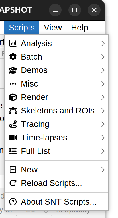
Scripts menu in main dialog
目前 SNT 中捆绑了 50 多个脚本。这些被组织成非严格的类别:分析(通常处理量化)、批处理(文件批量处理)、演示(教学示例)、渲染(可视化)、骨架和 ROI(基于像素的分析)、跟踪(跟踪相关任务)和延时(延时实用程序)。
可以通过两种方式访问捆绑的脚本:
- 主 SNT 对话框和 SNT 快捷方式窗口中的脚本菜单(选择脚本时按住 ⇧ Shift,以在脚本编辑器中打开它)
- 在脚本编辑器的Templates › Neuroanatomy › 列表中
您的脚本还可以与 SNT 捆绑在一起,或者通过 Neuroanatomy 更新站点提供。你写了一个有用的例程吗?请announce it,或提交pull request,以便可以在斐济分发!
添加脚本到 SNT
有几种方法可以让您自己的脚本出现在 SNT 的 Scripts 菜单中:
保存到 Fiji 的“scripts”子目录中且文件名中包含 SNT 的任何脚本(例如 C:\Users\user\Desktop\Fiji.app\scripts\My_SNT_Script.py 或 /home/user/Fiji.app/scripts/My_SNT_Script.py)都将在 Scripts 菜单中列出:
-
从 SNT 对话框转到 Scripts › New…。您可以选择使用您选择的脚本语言打开带有预加载样板代码的 Fiji 脚本编辑器实例,或者使用 Script Recorder 组装样板文件
-
将脚本保存在 Fiji.app/scripts/ 中,文件名中任意位置包含“SNT”
-
运行Scripts › Reload…,您的新脚本应该出现在Scripts › Full List…中的完整脚本列表中。
脚本记录器
SNT 具有一个脚本记录器,类似于_ImageJ 的宏记录器_,将菜单和按钮点击转换为可执行代码。但请注意,虽然记录器可以很好地捕获简单的命令,但它很难捕获更复杂或特别交互的命令。
记录器的目标有两个:1) 简化新脚本的原型设计;2) 记录跟踪会话期间的操作。这对于收集可重复的记录特别有用。
有两种方法可以启动录音机:Scripts › Record…或按Command Palette中的_Record_按钮。
根据经验,简单或不涉及提示的命令可以完美记录。这包括设置标签可见性过滤器、应用标签或在路径管理器中过滤路径。用于全自动重建或生成辅助层的命令应该可以很好地工作。然而,许多其他的仍然有限。
REPL
SNT 的脚本 REPL(读取-评估-打印循环)使用 Scripts › New › REPL 打开。它是一个具有预初始化变量的 Script Interpreter 实例,这些变量是当前 SNT 会话的 API 的入口点。 REPL 充当命令行提示符,可以访问所有 SNT 类。
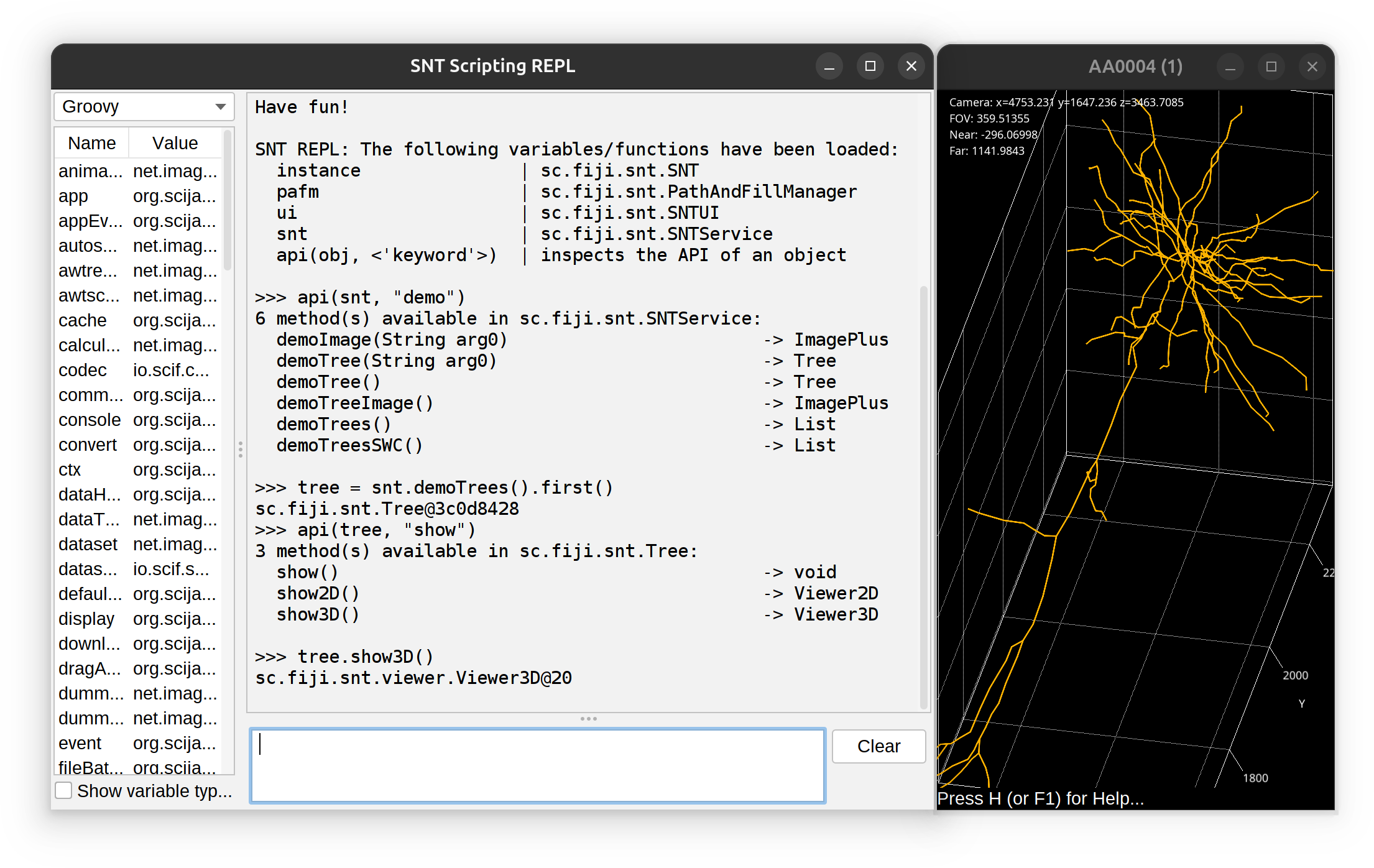
The REPL has access to all of SNT’s API. The prompt does not feature auto-completion but you can use api(object, 'optional keyword') to obtain a list of methods associated with an object. Example: To find out all of the ‘demo’ methods in SNTService, one would use:
>>> api(snt,“演示”)
sc.fiji.snt.SNTService 中有 7 种可用方法:
  demoImage(String arg0) -> ImagePlus
  demoImgPlus(String arg0) -> ImgPlus
  demoTree() -> 树
  demoTree(String arg0) -> 树
  demoTreeImage() -> ImagePlus
  demoTrees() -> 列表
  demoTreesSWC() -> 列表
外部数据分析
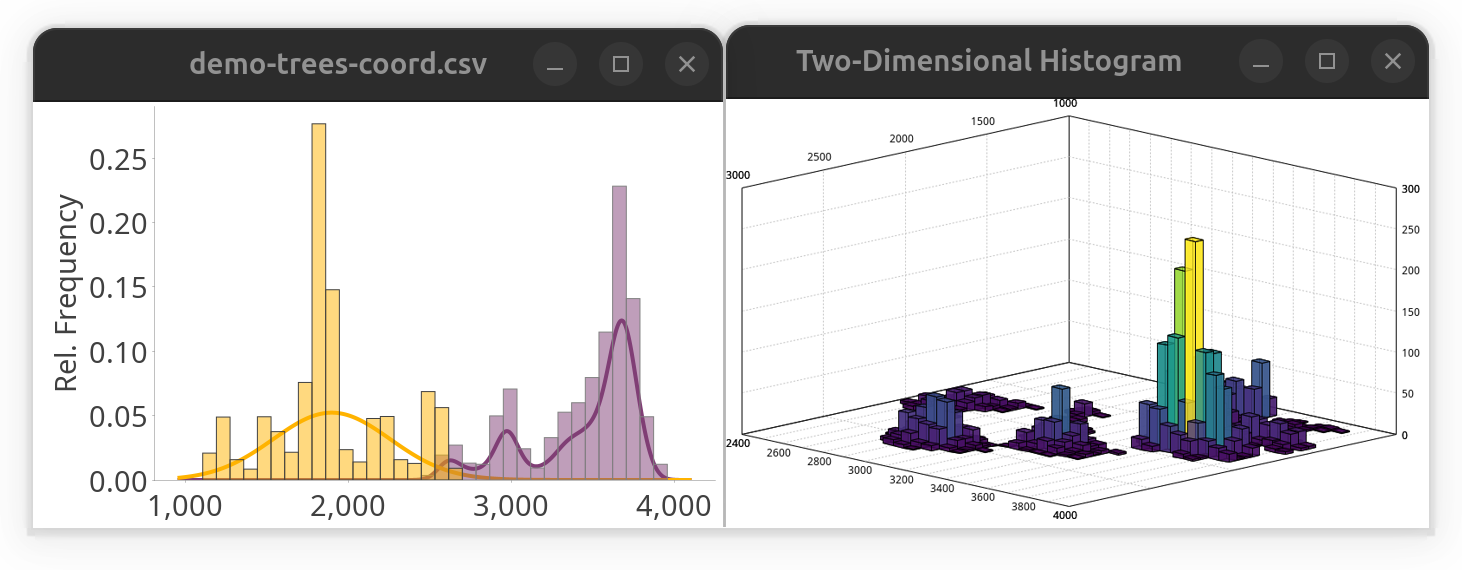
虽然SNT不是统计分析软件,但它确实提供了一些解析第三方数据的便捷方法。例如,要快速查看表格值的分布,可以使用以下代码片段来绘制直方图,同时将高斯混合模型拟合到数据。虽然它是用 Groovy 编写的,但它几乎可以在任何其他脚本语言中逐字运行,因为它仅依赖于 SNT API。
导入 sc.fiji.snt.analysis.*

path = "https://raw.githubusercontent.com/morphonets/misc/master/dataset-demos/csv/demo-trees-coord.csv" // 本地文件的 url 或路径
table = SNTTable.fromFile(path) // 将数据读入表中
headers = ["y", "z"] // 要绘制的列的标题
histogram = SNTChart.getHistogram(table, headers, false) // 表,列。标题,径向图?
histogram.setGMMFitVisible(true) // 将高斯混合模型拟合到数据
histogram.show() // 显示直方图
或者,可以将相同的数据绘制在二维直方图中:
导入 sc.fiji.snt.analysis.*
导入 sc.fiji.snt.util.*

path = "https://raw.githubusercontent.com/morphonets/misc/master/dataset-demos/csv/demo-trees-coord.csv" // 本地文件的 url 或路径
table = SNTTable.fromFile(path) // 将数据读入表中
SNTChart.showHistogram3D(table.get("y"), table.get("z"), ColorMaps.get("viridis")) // 使用 viridis LUT 显示相同列的 3D 直方图
请注意,此方法适用于本地和远程文件。两个片段并排的结果:
Python 笔记本
通过 PySNT 可以从 Python 编程语言直接访问 SNT API。这使得 SNT 与 Python 生态系统中的任何库(numpy、scipy 等)之间能够完全集成。 PySNT 的Tutorial Notebooks 包括多个不同复杂程度的教程。
斐济脚本
在斐济的脚本编辑器中编写脚本可能最好使用 Groovy 和 Python。后者对于非脚本参数的对象来说是非常好的自动完成功能。开始新脚本的最佳方法是在 SNT 中选择样板 Scripts › New › From Template… 或在脚本编辑器中选择 Neuroanatomy › Boilerplate。这些模板包含多种编程语言的样板代码(即BeanShell、Groovy和Jython),并包含最重要的导入和script parameters以促进快速开发。
更多资源
如前所述,SNT 的 source code repository 包括 Bundled Template Scripts 和 Jupyter notebooks。但网上确实存在其他片段、示例和进一步的教程,包括:
例子
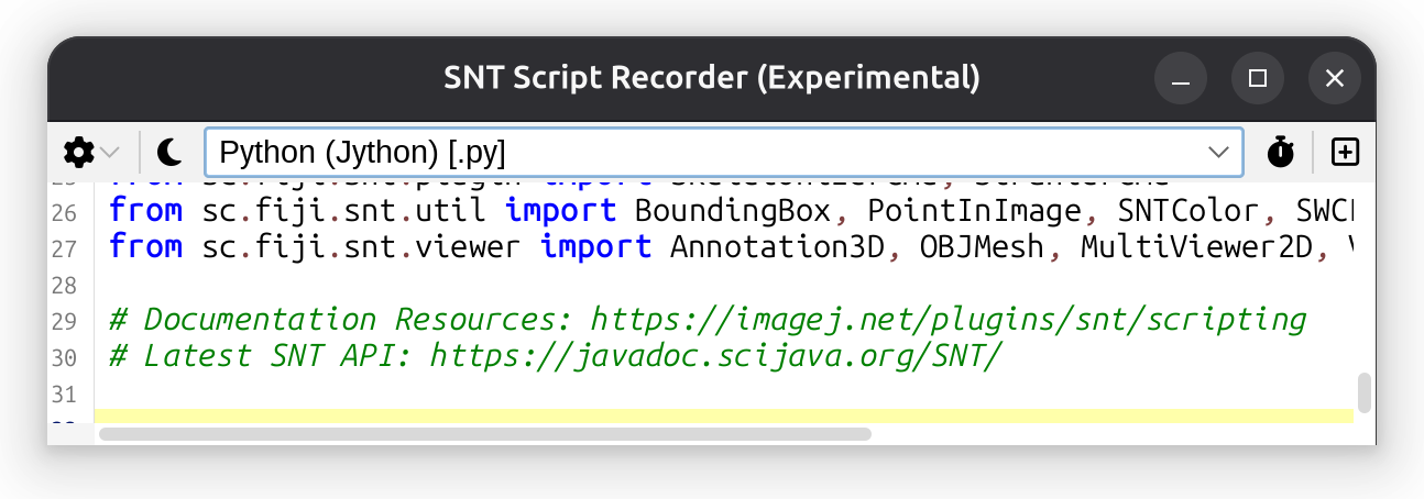
通过选择 Scripting › Record Script… command 可以实现对 Reconstruction Viewer 的开放实例(从 SNT 内调用或作为独立应用程序调用)的编程控制。然后,它将打开一个 SNT 脚本记录器的实例,其中加载了包含最基本的导入和script parameters的样板模板。该模板的默认编程语言可以从记录器的下拉菜单中选择。
以下脚本示例了如何扩展样板模板以实时控制查看器。
# 最后测试:2024-07-12,SNTv4.3.0pre
#@上下文上下文
#@DatasetService ds
#@DisplayService显示
#@ImageJ ij
#@LogService日志
#@LUTService lut
#@SNTService snt
#@UIService 用户界面

从 sc.fiji.snt 导入路径、PathAndFillManager、SNT、SNTUI、树
从 sc.fiji.snt.analysis 导入 GroupedTreeStatistics、MultiTreeStatistics、NodeStatistics、TreeStatistics、\
            ConvexHullAnalyzer, PersistenceAnalyzer, ShollAnalyzer, StrahlerAnalyzer, NodeColorMapper,\
            TreeColorMapper, PathProfiler, PathStraightener, RoiConverter, SkeletonConverter, SNTChart, SNTTable
从 sc.fiji.snt.analysis.graph 导入 DirectedWeightedGraph
从 sc.fiji.snt.analysis.sholl.parsers 导入 TreeParser
从 sc.fiji.snt.annotation 导入 AllenCompartment、AllenUtils、VFBUtils、ZBAtlasUtils
从 sc.fiji.snt.io 导入 FlyCircuitLoader、MouseLightLoader、NeuroMorphoLoader
从 sc.fiji.snt.plugin 导入 SkeletonizerCmd、StrahlerCmd
从 sc.fiji.snt.util 导入 BoundingBox、PointInImage、SNTColor、SWCPoint
从 sc.fiji.snt.viewer 导入 Annotation3D、OBJMesh、MultiViewer2D、Viewer2D、Viewer3D

# 文档资源:https://imagej.net/plugins/snt/scripting
# 最新 SNT API:https://javadoc.scijava.org/SNT/

# 推荐。查看器 API:https://javadoc.scijava.org/SNT/index.html?sc/fiji/snt/viewer/Viewer3D.html
# 提示:场景详细信息可以使用 `viewer.logSceneControls()` 打印到控制台或记录
# 当查看器位于最前面时按“L”(助记符:[L]og)
# 如果从独立 RV 打开此模板,则为查看器的实例 ID(例如 2)
# 将自动作为参数传递给 getRecViewer()
查看器 = snt.getRecViewer()

# 添加的代码从这里开始 ####################################################################
导入时间

def do_stuff(查看器):
    viewer.logSceneControls()

    # Load a neuron from Mouse Secondary Motor Area from the MouseLight database.
    loader = MouseLightLoader("AA0100")
    if not loader.isDatabaseAvailable():
        ui.showDialog("Could not connect to ML database", "Error")
        return
    if not loader.idExists():
        ui.showDialog("Somehow the specified id was not found", "Error")
        return

    # Extract nodes with tag "axon".
    axon = loader.getTree('axon')
    # Do the same for the dendrites.
    dendrites = loader.getTree('dendrites')

    # Load the Allen CCF Mouse Reference Brain and add it to the scene
    viewer.loadRefBrain('mouse')

    # Add both Trees to the scene
    viewer.addTree(axon)
    dendrites.setColor('cyan')
    viewer.addTree(dendrites)

    # Get the OBJMesh object representing the maximum depth Allen CCF compartment
    # containing the soma point and add it to the scene.
    soma_annotation = loader.getSomaCompartment()
    viewer.addMesh(soma_annotation.getMesh())

    # Enforce side perspective.
    viewer.setViewMode('side')

    # Next, we will apply a color mapping to the axon
    # using branch order as the metric and the Ice Lut.
    # Make an instance of TreeColorMapper using SciJava context.
    mapper = TreeColorMapper(context)
    # Get the net.imglib2.display.ColorTable object.
    lut = mapper.getColorTable('Ice.lut')
    # Color code the axon and render in scene.
    # The min and max values returned by the mapper are used
    # to set the range of the color bar legend.
    bounds = viewer.colorCode(axon.getLabel(), TreeColorMapper.STRAHLER_NUMBER, lut)
    viewer.addColorBarLegend(lut, bounds[0], bounds[1])
    # Display a text annotation of the cell ID and metric used by the mapper.
    scene_annotation = "{}: Branch Order".format(axon.getLabel())
    viewer.addLabel(scene_annotation)

    # Begin a rotation animation for the objects in scene.
    viewer.setAnimationEnabled(True)
    # Wait some time before applying a new color mapping
    # based on path distances, using a different LUT (Fire).
    time.sleep(5)

    lut = mapper.getColorTable('Fire.lut')
    # Remap the axon Tree and update scene.
    bounds = viewer.colorCode(axon.getLabel(), TreeColorMapper.PATH_DISTANCE, lut)
    viewer.addColorBarLegend(lut, bounds[0], bounds[1])
    scene_annotation = "{}: Path Distance".format(axon.getLabel())
    viewer.addLabel(scene_annotation)
do_stuff(查看器)批量生成过滤图像
本节介绍如何在 SNT 之外批量生成 Filtered Images。请注意,该主题有 many tutorials。可以说,处理多个图像的最简单方法是 1) 记录一个处理单个图像的宏,然后 2) 将其包装在一个循环中以迭代目录中的所有文件。例如,使用IJ1宏语言:
d = getDirectory("选择目录");
文件= getFileList(d);
扩展名=“.tif”;

for( i = 0; i < 文件长度; ++i ) {
    filename = files[i];
    if( endsWith(filename,extension) ) {
        l = lengthOf(filename);
        el = lengthOf(extension);
        basename = substring(filename,0,l-el);
        expected_window_name = "result";
        output_filename = d + File.separator + basename + ".tubes.tif";
        open(filename);
        run("Gaussian Blur...", "sigma=2 scaled stack"); // processing step here
        selectWindow(expected_window_name);
        saveAs("Tiff", output_filename);
    }
}
使用 ImageJ Ops 在脚本中可以更完整地完成相同的过程。例如,在 Jython 中: