特拉克EM2

自迁移出 MediaWiki 以来，本页内容尚未经过审查。如果您愿意帮忙，请查看帮助指南！

TrakEM2 是一个 ImageJ 插件，用于形态数据挖掘、三维建模和图像拼接、配准、编辑和注释。

有关概述，请参阅TrakEM2 snapshots。

特点

• 分割：手动绘制堆栈上的区域，并用球和管道绘制结构草图。骨架化整个神经元树枝化并用关系连接器对象表示突触。
• 测量：体积、表面、长度以及通过 ImageJ ROI 进行的测量。
• 图像配准：使用SIFT和全局优化算法相互配准浮动图像图块。
• 3D 可视化： 与 3D Viewer 插件交互，TrakEM2 显示图像体积和各种 3D 网格。
• 图像注释：浮动文本标签。
• 语义分割：树层次结构中的顺序分割，其模板可导出以在其他类似项目中重用。

TrakEM2 与 3D Viewer 交互以实现图像体积和 3D 网格的可视化。

斐济的 TrakEM2

• 从“文件 - 新建 - TrakEM2（空白）”创建新项目
• 通过将 .xml 文件拖到工具栏上或通过“文件 - 打开”来打开现有项目。

文档

• How to
• Manual
• TrakEM2 tutorials 带有视频教程。
• scripting in TrakEM2的示例。
• 写作plugins for TrakEM2。

运行 fiji 来执行重型、内存密集型、高性能 TrakEM2 任务

以下配置已在具有 256 个 CPU 核心和 1 TB RAM、运行 Ubuntu 22.04、最新 1.8.0 JVM 的机器上进行了测试：

-Xms500g -Xmx500g  -XX:+UseG1GC -verbose:gc -XX:+PrintGCDateStamps

鉴于 Fiji 使用增量垃圾收集器（通过 -Xincgc）启动，而不是并发垃圾收集器（通过上面的 -XX:UseG1GC），您不能像更新 RAM 使用情况那样修改 ImageJ.cfg 文件（通过 -Xms500g -Xmx500g）。相反，请执行以下操作：在终端中生成一个试运行命令，将其通过管道传输到文本文件中，对其进行编辑以替换 G1 GC 的 -Xincgc，使文件可执行，然后启动它。这个 sed 脚本也可以做到这一点：

$ ./ImageJ-linux64 --dry-run | sed 's/-Xincgc/-XX:+UseG1GC -verbose:gc -XX:+PrintGCDateStamps'/ >> launcher.sh
$ chmod +x launcher.sh
$ ./launcher.sh

JVM 标志的含义：

• -Xms500g ：使用 500 Gb 的初始堆大小（即以预先分配给它的 500 Gb RAM 启动 fiji）
• -Xmx500g：使用最大堆大小 500 Gb。请注意，它与初始堆大小相同，因此无法调整堆大小。
• -XX:+UseG1GC ：使用并发垃圾收集器。使用并行线程清理未使用的内存。 –verbose:gc：可选，查看垃圾收集器何时运行。
• -XX:+PrintGCDateStamps：查看GC何时运行的记录。

通过上述设置，我们已经在 TrakEM2 中成功注册了数万个切片和数百万张图像。

准备 TrakEM2 以获得最佳性能

以最快的速度浏览图层

右键单击画布并选择“显示 - 属性…”。然后确保：

• “快照模式”设置为“禁用”，或最多设置为“轮廓”。
• 未选中“预绘制”，因此它被禁用。

用于导入大量图像并随后立即编辑它们

目标是避免多次生成 mipmap，这可能非常耗时。

右键单击画布并选择“显示 - 属性…”。然后确保：

• 未选中“启用 mipmaps”，因此它被禁用。

请注意，导入时您将无法快速浏览图层，因为不会生成 mipmap。

现在要校正对比度，首先重新启用 mipmaps，方法是再次转到“显示 - 属性…”并选中“启用 mipmaps”复选框。然后你有两个一般（非排他性）选项：

A. 使用右键菜单中的内置命令，例如：

• “调整图像 - 逐层增强对比度”
• “调整图像 - 逐层设置最小和最大”

B. 创建预处理器脚本并将其设置为所有图像。例如，在每个图像上运行 CLAHE 的 beanshell 脚本。在脚本中， patch 和 imp 变量自动存在，并分别表示 Patch 包装的 Patch 实例和 ImagePlus 实例。

import ij.IJ;
IJ.run(imp, "Enhance Local Contrast (CLAHE)", "blocksize=127"
   + " histogram=256 maximum=3 mask=*None* fast_(less_accurate)");

要将脚本设置为所有图像，请将上述内容保存到名为“whatever.bsh”的文件中（注意文件扩展名“.bsh”），然后右键单击 TrakEM2 画布并选择“脚本 - 设置预处理器脚本逐层”，然后选择整个图层范围。这会将脚本设置为每个图层的每个图像，并触发每个图像的 mipmap 重新生成。当 TrakEM2 加载图像时，脚本将在 TrakEM2 查看其内容之前在图像上运行。

预处理器脚本为您提供了最大的能力：对图像执行任何您想要的操作。例如， normalize the image 相对于数据集的已知良好平均值和标准差。

以最快的速度重新生成 mipmap

mipmap 的默认生成是通过平均完成的，并且速度相当快。不过，您可能需要考虑并行化它：转到“项目 - 属性…”，并将 mipmap 线程设置为计算机中的核心数，例如 12。

如果您对 TrakEM2 中缩放图像的默认质量感到满意，请停止阅读。

如果您选择使用高斯生成 mipmap，请转到“项目 - 属性…”，并将 mipmap 模式设置为“高斯”。然后，您必须注意以下事项：

在 TrakEM2 0.9a 及更高版本中，mipmap 机制可以使用最新 ImageJ 中现有的多线程高斯实现。这意味着现在有两组线程：

1. 线程集，其中每个线程重新生成单个图像的 mipmap 金字塔。
2. 对于生成 mipmap 金字塔时的每次缩放迭代，执行高斯模糊以进行下采样的线程集。

如果您的机器有 12 个核心，则默认设置将使用 1 个线程进行 mipmap，使用 12 个线程进行高斯模糊。这可能不适合您的数据属性：如果您的图像很小，您最终可能会等待很长时间来生成 mipmap。

有两种策略可用于加速基于高斯的 mipmap 生成：

• 策略A：您的数据由大图像组成（超过4000x4000）。右键单击 TrakEM2 显示屏并选择“项目 - 属性…”，然后将 mipmap 线程设置为 1（默认值）。现在，将一次为一张图像重新生成 mipmap，使用 12 个线程（给定 12 个内核）来计算高斯分布。
• 策略 B：您的数据由小图像组成（小于 4000x4000）。转到 Fiji 窗口并选择“编辑 - 选项 - 内存和线程…”，并将线程数设置为 1。然后，转到“项目 - 属性…”，并将 mipmap 线程设置为 12。现在，将一次为 12 个图像重新生成 mipmap（给定 12 个核心），每个图像使用一个线程来计算高斯。

如果您的计算机 RAM 很小，或者对图像的访问速度缓慢且有争议（例如数据位于 USB 硬盘驱动器中），也请使用策略 A。这就是为什么默认使用一个单线程来生成 mipmap。

如果将生成mipmap的方法更改为非高斯方法，则不会出现上述情况。将用于重新生成 mipmap 的线程数设置为核心数，如果您的计算机没有太多 RAM，则设置更少。

使用更大的四叉树桶，XML 加载速度更快，内存消耗更少

除了为大图像选择合适的 mipmap 生成策略之外，还要确保正确设置存储桶大小。

TrakEM2中什么是桶：每一层（每个部分）都有一个内部Quadtree，能够找到鼠标下的物体（例如图像），或者能够快速找到与其他图像重叠的图像。换句话说，能够执行快速空间查询，例如查找与给定矩形相交的所有图像的列表。

如果存储桶尺寸很小（默认边长为 4096 像素，那么一个存储桶就是一个 4096x4096 像素的正方形，可以认为非常小），那么与非常大的画布尺寸相结合，将会生成太多的存储桶。 会花费大量时间并且消耗大量内存。

如果您的每个部分只有大约 100 个图像，并且图像有些大（例如，每个图像的尺寸为 8096x8096 像素），则将存储桶大小设置为比默认值大得多的值，例如 100000。实际上只有一个存储桶。

当图层中有许多小对象或许多可显示的小对象时，小存储桶就有意义。在这种情况下，例如每层只有一个图像，但其上有许多较小的 Ball 或 Pipe 或 AreaList 对象，则采用默认存储桶大小 (4096) 或更小。否则，选择大的甚至非常大的，有效地删除存储桶功能并减少列表搜索，这对于像大约 100 个这样的小图像列表来说就很好了。

当注册/对齐分布在 5,000 个部分的 400,000 个图像的集合时，使存储桶变大是有意义的（例如 40960，默认值的 10 倍，甚至比该值更大）。 将存储桶大小设置为较大的值将减少 XML 加载时间大量。

要设置存储桶大小，请右键单击并选择“显示 - 属性…”并写入存储桶大小值。

我应该为 Fiji 的 JVM 分配多少 RAM 来运行 TrakEM2？

使用遵循以下经验法则的计算机：获取数据集中最大的单个 2D 图像，然后将其大小乘以 10，并确保 CPU 的每个核心至少有那么多可用的 RAM。

例如，对于 4096x4096 16 位图像，每个核心至少需要 335 Mb，因此 16 个核心至少需要 5.4 Gb RAM。 8 GB 可能会更好。 32 GB 使用起来很愉快。

至于显卡，请购买您能负担得起的最大显卡，无论是计算能力还是内存。

示例

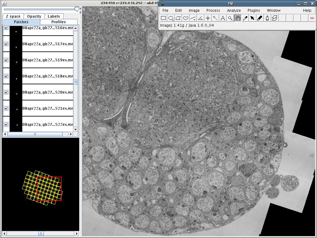TrakEM2: 359 montages of 13x13 tiles of 2048x2048 pixels each.

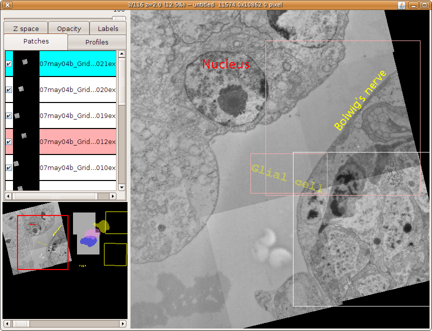fig:TrakEM2 Display showing 9 images in a layer, where 2 images and one floating text label (set to 30% transparency) are selected (pink and white frames; white is the active one – note the corresponding pink and blue coloration of the object panels on the left). The Navigator (bottom left) paints a red frame to indicate the area currently displayed in the canvas (right).

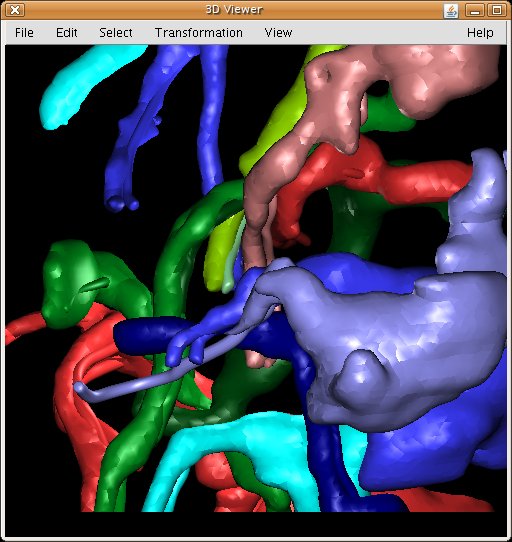3D Viewer: hardware-accelerated 3D visualization of image stacks as volumes, orthoslices and meshes. Above, secondary lineages of Drosophila third instar larval brain segmented in TrakEM2.

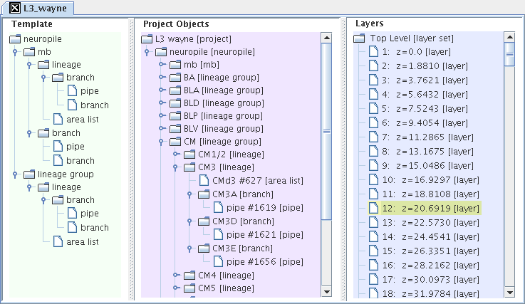The three TrakEM2 trees, as an interface for editing and visualizing the three internal TrakEM2 data structures.

Effect of the CLAHE live filter in TrakEM2. Data with high dynamic range is displayed with perceptually boosted local contrast. CLAHE parameters are relative to display pixels and, therefore, will not result in an effective bandpass when zooming out largely on statically pre-processed images.

Neuronal arbors reconstructed with TrakEM2 using the treeline segmentation type.

Neuronal arbors from serial section electron microscopy reconstructed with TrakEM2 using the manually segmentated data set.

TrakEM2 showing one section of a serial section transmission electron microscopy (ssTEM) data set, with numerous neuronal arbors reconstructed using treelines and connectors (for synapses).

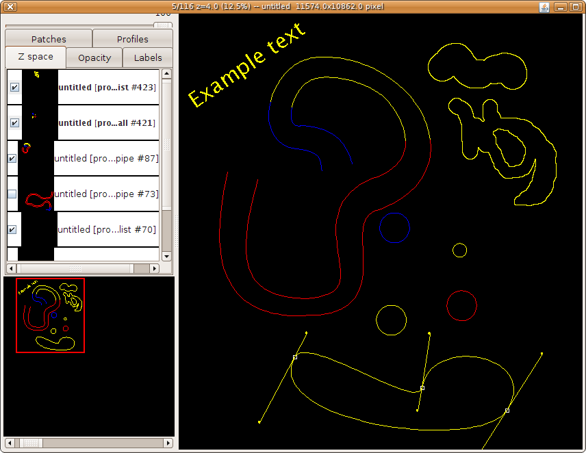Example TrakEM2 segmentations, including Ball, Pipe, Profile, AreaList and floating text labels.

出版

doi:10.1371/journal.pone.0038011