自迁移出 MediaWiki 以来，本页内容尚未经过审查。如果您愿意帮忙，请查看帮助指南！

简介

Watershed [Vincent 1991] 是分割 2D 和 3D 图像中对象的常用工具。它相对较快，可以提供可理解且可靠的结果，可用于图像分析。

然而，创建良好的正确解析需要一些专业知识，并且可能非常运行。必须人们确定的阈值来阻止分水岭。必须选择有意义的局部极值来启动算法。一旦获得结果，就必须将分割与原始数据进行比较。然后可以迭代该过程直到找到满意的参数。如果没有提供实用工具，该过程可能会非常顺利，尤其是当图像很大且单个分水岭可能需要数百的时间时。

洪水分水岭插件提供了一种洪水方式来探索局部（顶部）和阈值，动态更新生成的分水岭。这是可以通过在插件初始化时计算一次分水岭来实现的。此外，当阈值或立即选择更新时，该初始分割将被重新使用以生成新的分割。为了以此质量评估，结果直接到数据上。

以下第2小节提供了有关分水岭工作原理以及局部顶峰检测插件中使用的策略的更多详细信息：H-Maxima

分水岭原理

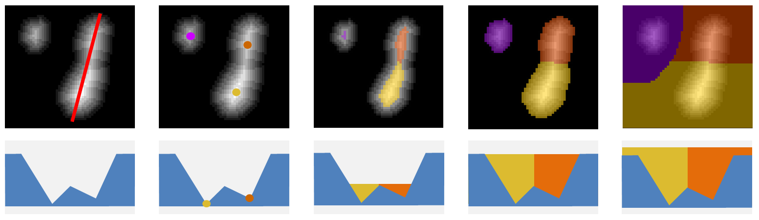
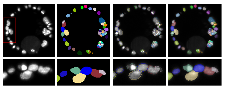
如果我们将图像解释为丘陵和山谷的地貌，则图像分水岭算法从山谷的最低点（图像局部稀疏）开始逐渐淹没水平。当两个不太明显的洪水在鞍点处相遇时，它们仍然不同，因为每个区域都标有不同的颜色。当所有图像被覆盖时，泛滥。停止由于对象并不总是覆盖整个，可以设置阈值来阻止区域泛泛。或者，从可以局部端点开始泛洪。图2显示了不同的阈值参数值的3个热门的泛滥。

H-极大值和H-分水岭

图像中的多个顶点只是由噪声引起的，没有意义。如果可以选择与对象相对应的更重要的顶点，则利用它们来启动这些对象的分水分割。

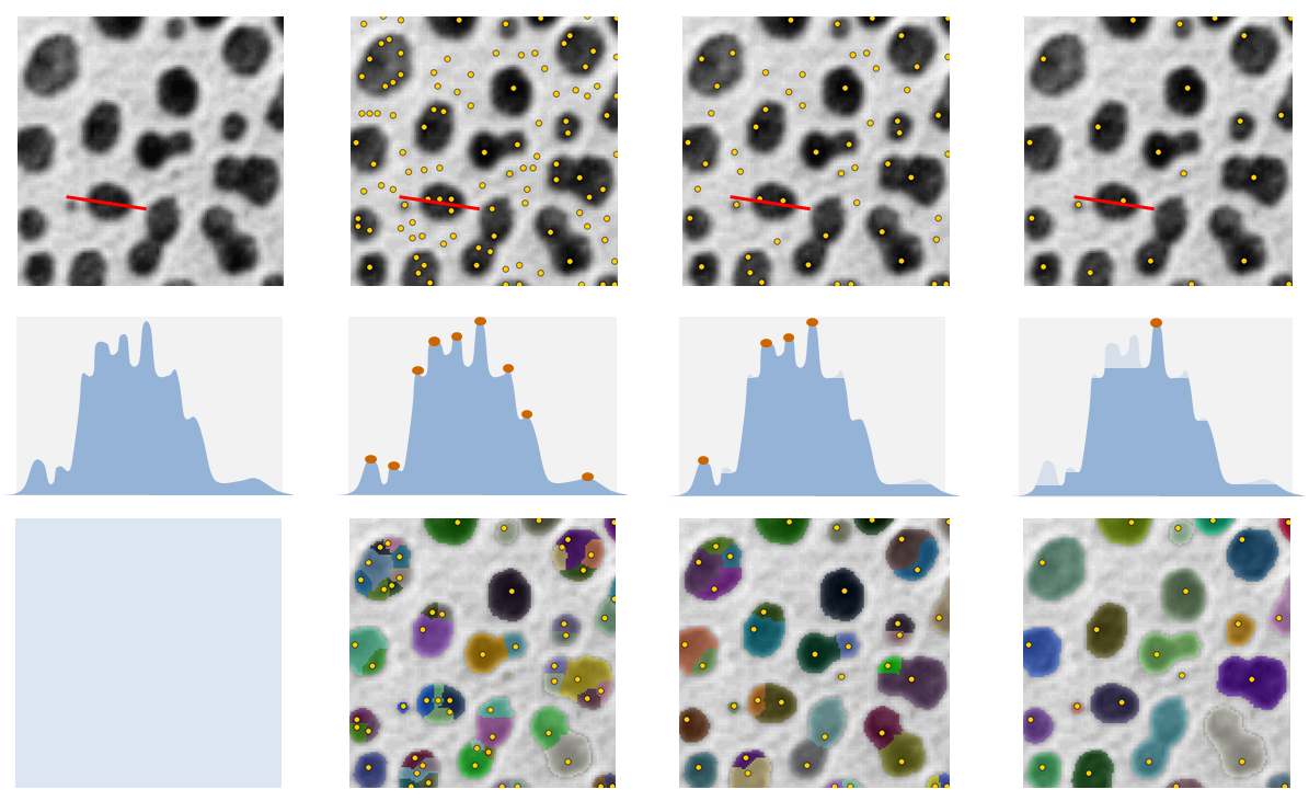
存在多种检测局部顶峰的方法。H-maxima关注最大鲁棒性。它有一个参数H，可以与图像中噪声的幅度进行比较。H-maxima选择所有的顶峰，当它们的值减少H时，这些顶峰仍然是顶。当H增加时，选择的顶峰会减少，但它们最终对噪声更加鲁棒。图3在示例中显示了针对不同H值选择的顶峰。

我们将通过淹没图像的 H 顶峰而获得称为 H 分水岭的分割。这种分割有 2 个参数。停止图像泛洪的阈值 T 并定义泛洪初始化的 H 顶鲁棒性 H。

方便

安装

在 ImageJ 或 Fiji 安装中安装该插件。添加更新站点SCF-MPI-CBG。如果还没有 Java8 更新站点，也应该安装它。按照更新站点的程序can be found there。

安装更新站点后，重新启动ImageJ。应该会出现一个新菜单SCF。交互式分水岭插件可以在菜单 SCF>Labelling>Interactive H_Watershed 中找到。

用户界面

使用吸引力分水岭插件。

1.打开图像进行分析。如果图像有多个通道或时间点，则切除出单个通道/时间点。该插件集中于分析2D和3D图像。

1. 在菜单 SCF>Labelling 中单击项目 Interactive H_Watershed。该插件将使用焦点图像进行初始化。然后执行图像的完整水。如果很大，将弹出一个处理指示，指示剩余时间。如果可以需要，中断该过程。在这种情况下，您可以缩小较小的体积并重新启动。 3.初始化后会弹出2个窗口：分水岭图像和控制面板。当控制面板修改时，分水岭图像会立即更新。对分割满意后，按导出按钮创建标签图。

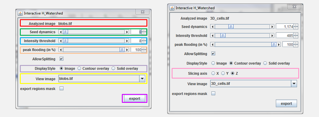
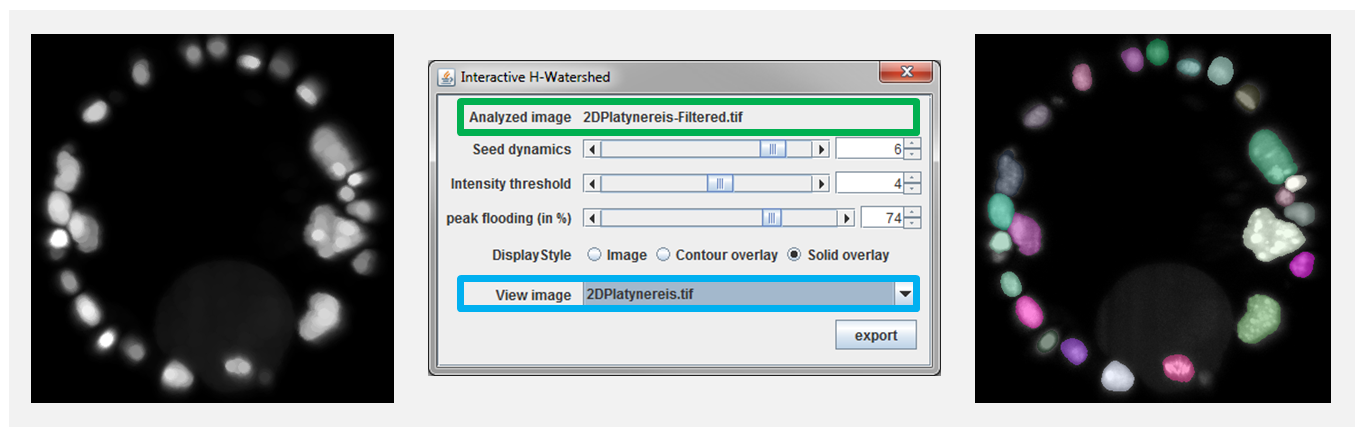
控制面板项（参见图4）可用于修改显示屏及其可视化。本节的其余部分描述了它们的用途：

• 分析图片：这是图片分析的名称。这是用于用户信息的
• 分割参数：
  • Seed dynamics: The slider allows to adjust the H-maxima selection. Increasing that value will merge regions, while decreasing it will split regions. Note that the value shown at the end of the line is not the actual \(H\) but \(log(1+H)\). The reason is that logarithm scale provides a more intuitive interaction (many merging happen at low \(H\) but much fewer at large \(H\).
  • Intensity threshold: The slider allows to select the watershed stopping criteria, \(T\). Increasing \(T\) decreases regions size while decreasing \(T\) till they eventually disappear. Note that the value shown at the end of the line is not the actual \(T\) but \(log(1+T)\). Logarithmic scale provides a more intuitive interaction as regions usually evolve fast for low \(T\) but much slower for larger \(T\).
  • Peak flooding: this parameter is an alternative way to explore regions thresholds. Rather than using a global threshold one can apply distinct thresholds to each segment. Peak flooding allows to flood each peak till a certain percentage of its height. For the region \(i\) the threshold \(T_i = T + \alpha/100 . (Imax_i-T)\), where \(T\) is the threshold parameter, \(\alpha\) is the peak flooding in percent and \(Imax_i\) is the maximum intensity in region \(i\).
  • Allow Splitting: if checked, playing with threshold or peak flooding might create new region by splitting existing one. If allow splitting is not checked the no new region is created, only the peak with the highest maxima is kept.

• 显示参数：
  • Display style decides how the current segmentation is displayed. The different modes are illustrated in Figure 5.
    • Image will show directly the label map of the segmentation. This mode is convenient to adjust the segmentation display control and look up table with imageJ usual tools.
    • Contour overlay mode overlays regions contours to a background image (by default the analyzed image). This mode is very convenient to check that the regions shape match object shape in the raw data.
    • Solid overlay mode overlays solid segment to the background image.
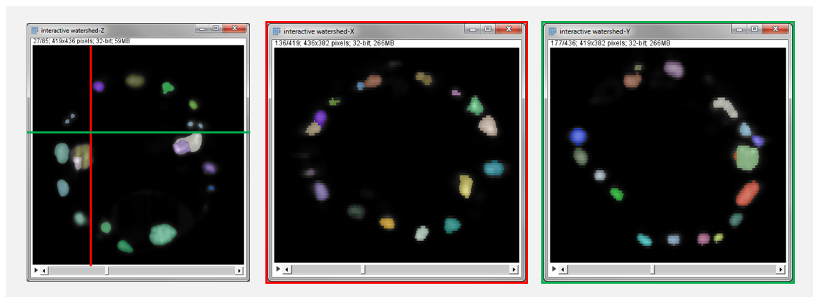
  • Slicing axis: If the analyzed image is 3D the user can select the orientation of the result visualization. Selecting X will slice the data in the plane perpendicular to the X axis (the plane YZ). As the resolution of microscopy data is often lower in the Z dimension and might be the bottleneck for segmentation quality it is important to check segmentation quality in plane XZ and YZ. The choice of slicing axis is illustrated in figure 6. By default the result window show XY planes. Navigation through the planes is done with usual ImageJ controls (image slider, mouse wheel, arrows).
  • View Image selects the background image (i.e. shown below the segmentation overlay). By default, it is the image that was segmented, but can also be set to any other image with the same dimension. Note that images can’t be added to the list after plugin initialization. This feature is practical to compare region shape to the original data. For instance, if the segmentation was done on a filtered image that could have alter object shape (see figure 7).
• 导出区域蒙版：如果选中导出按钮，将导出二进制图像而不是标签图像。如果图像是 2D，则该二值图像与 ImageJ 的颗粒分析仪兼容。
• 导出：一旦对屏幕上可见的分割感到满意，就可以将相应的标签图导出到 ImagePlus，以便使用 ImageJ 进行进一步分析。导出操作出现在图像宏语言和 Jython 语言的宏记录器中。

脚本编写

在 ImageJ 宏语言中，可以使用以下命令执行 H-Watershed 分割：

在 Jython 脚本中，H-Watershed 部分可以按如下方式调用：

导出标签映射时，宏记录器基因记录运行命令。

方法与实现

该插件是在策略开始时执行一次繁重的工作，然后依靠它来保持分段更新的轻量级别。

重物搬运

在初始化时，插件计算图像的完整分水岭（即形成图像的所有局部顶点）。然后以自下而上的方式组织该深入解析。这些部分逐渐合并以层次结构（如果您愿意，也可以形成树）。首先，合并其顶点具有最低动态（或最低鲁棒性，记住H）顶）的分段。当两个段合并时，它们的动态和相邻段的动态将被重新评估。重复此合并过程，直到合并所有段。它生成一棵树，其节点对应于图像中的分段。特别是，当沿树枝从叶子到根时，节点的动态总是增加。

这个过程的结果，我们获得了完整的分水岭标签图并表示标签作为区域合并的树。

分割的轻量级更新

当 H 参数更新为值 \(h\) 时。这意味着分水岭应该只显示局部顶端的动态补偿 \(h\) 的部分。如果我们修剪整棵树以删除动态性低于 \(h\) 的所有节点，则修剪后树的叶子对应于我们正在寻找的部分。我们现在需要整个分水岭的标签图重新对着色，以创建具有 \(h\)-maxima这可以通过为稀疏岭树的叶节点添加标签来完成。然后包裹标签传播到原始树的叶节点。最后，完整分水的部分可以根据这个新标签重新着色。整个过程非常：快速标记是原始标签图上的简单栅格传递，并且树的节点数比中的像素数少很多。

当T参数更新时，顶点不会被修改，因此只需遍历标签图并检查原始数据中的像素值是否为某个或低于阈值。当洪水参数改变时，策略类似，但每个段作为不同的阈值

对实施的评论

根据我们同样，使用热门动态作为合并标准的分水岭段层次结构的最初描述在[Najman 1996]中进行了描述。该插件最初分水是在IFT-分水岭[Lotufo 2000]实现的。修改了实现以动态构建线段树。插件输入和输出是IJ1 imagePlus，但内部的图像处理依赖于ImgLib2。关于3D图像分割更新的快速说明，该插件不会在每次更新时重新标记整个体积，而只是对可视化的切片进行重新标记，以保持交互性。

参考文献

[文森特 1991] 文森特，L.，＆苏耶，P.（1991）。数字空间中的分水岭：基于沉浸模拟的算法。IEEE模式分析和机器智能交易，13(6), 583-598。

[Najman 1996] Najman, L. 和 Schmitt, M. (1996)。分水岭构建的测地线显着性和分层分割。IEEE 模式分析和机器智能刊汇，18(12), 1163-1173。

[Lotufo 2000] Lotufo, R. 和 Falcao, A. (2000)。社区队列和分水岭逼近的最优性。在数学形态学及其在图像信号和处理中的应用。

历史

SCF_MPI_CBG 更新站点的可用版本历史记录

• 2017-05-11：版本1.0.0
  • inital release

• 2017-06-12：版本1.0.1，
  • features: smoother slider for threshold and seeds
  • bugFix: correct initialisation of the segmentation in the script call (this correction suppress discrepency between the GUI and the script call)

• 2017-07-03：版本1.0.2
  • feature: the labelling is always continuous from 1 to number of labels in the image/volume
  • feature: threshold and seeds dynmics slider range fix to [0,1000] with step of 1
  • bugFix: the exported label map shows the correct number of labels in its title
  • bugfix: threshold value in in output title corrected

• 2017-08-16：版本1.0.4
  • feature: in scripting the parameter are optionnal (defaults, thresh = min , seed dynamics = 0.05*(Max-Min) , peakFlooding = 100). See jython script on the project repository for usage details.
  • bugfix: the output image is not a virtual stack anymore. That was annoying for further analysis of the regions.
  • bugfix: The output image now the same calibration as the input

• 2017-08-17：版本1.0.5
  • bugfix: correct a regression with the macro recording.

• 2017-09-21：版本1.1.0
  • Add the possibility to export a mask that can be directly analyzed with the particle analyzer. the run(…) or IJ.run(…) were updated to reflect the additional parameter

• 2018-01-10：版本1.2.1
  • this version corrects a long standing bug such that object could be splitter by changing threshold while the 2 new region kept the same labeling. now the new regions are either relabeled either only the highest remaining region is kept. the choice is made depending on allow splitting parameter.
  • the exported image is not a virtual stack anymore avoiding issue with further processing
  • the exported image name is also updated the reflect more faithfully the name of the input image
  • the threshold and seed slider are now linear: as a result the value displayed in the user interface is directly related to image intensity. which make parameter reading easier.