

通过互相关进行共定位
该插件尝试确定:非随机空间关联粒子之间的平均距离、该距离的标准偏差(对于衍射受限图像,该距离还应反映图像中 PSF 的宽度)以及关联的两个统计度量。它通过在两个图像之间执行互相关函数 (CCF) 来实现此目的,其操作方式与 Van Steensel 的 CCF 类似,不同之处在于该插件在所有方向上执行 CCF 并提供附加信息,例如标准差和统计测量。它目前适用于 2D/3D 单通道图像,支持时间序列分析,并需要对其中一幅图像中的信号的所有可能定位进行掩码。
安装插件:
可在 ImageJ updates sites 列表中找到。需要斐济。
如何使用互相关共定位 (CCC):
简要概述
- chromatic shift正确
- 准备要分析区域的掩模
- 对图像进行反卷积(可选但推荐)
- 将图像转换为 32 位(图像 > 类型 > 32 位)
- 测量并减去两个图像的平均背景(处理>数学>减去)
- 验证精确缩放(图像 > 属性)
- 运行插件
为像素随机化准备一个掩码
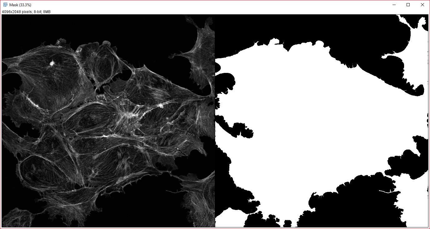
Analysis mask: An example of an appropriate mask for analyzing cross-correlation of cytoplasmic proteins(right), generated from an actin stain (left).
To get the best possible results, you will want to create and save a segmented mask for one of your images. This should be a mask of where within the image your want to search for spatial correlations. Generally, the mask should contain all possible localizations for your stains or dyes, or it should be a mask of localization for your null hypothesis (i.e if you hypothesize a protein is localized to the mitochondria, you would want your mask to encompass the entire cell). As an example, say you are studying correlation between two nuclear proteins, then you would want your mask to cover the nucles, which could be created easily using a DAPI or Hoechst stain (the mask itself does not need to be generated from either image your are trying to correlate). If you were studying cytoplasmic proteins, you would want your mask to cover the entire cytoplasm. The mask is very important and not using it could easily lead to undesired correlations. This is because without a mask this plugin will find correlations at any distance, and, if say you are studying nuclear proteins, can easily correlate one nuclei to the nuclei of a neighboring cell (cells are often highly repetitive and spaced relatively evenly). This broad correlation is the low spatial frequency component, and if not corrected for your results will be affected by it. However, when an appropriate mask is used, these cell to cell correlations will be subtracted out during the analysis.
Prepare your images
Deconvolving your input images can drastically improve the results of CCC and is highly recommended.
It’s also best to use an appropriate background subtraction method on the two data images in order to lower the background pixel values. While pixels outside of the masked region do not contribute to the cross-correlation result, having a high signal to background ratio within the masked region will help improve the confidence signifiantly. Images should be converted to 32-bit depth prior to background subtraction. This should be done to allow negative values in the image, which will improve the results of the statistical measure. After converting to 32-bit, the mean background value, measured from a region devoid of signal, should be subtracted from the image. For 3D images where the majority of voxels are background, you can use the search bar to run the ‘stats.median’ ops function, which will give you an appropriate background value for the entire image.
Additionally, the images (particularly 3D) need to be correctly scaled (Image > Properties), otherwise all axes will be assumed to have the same scale and your mean correlation distance will be in pixels.
Run the plugin
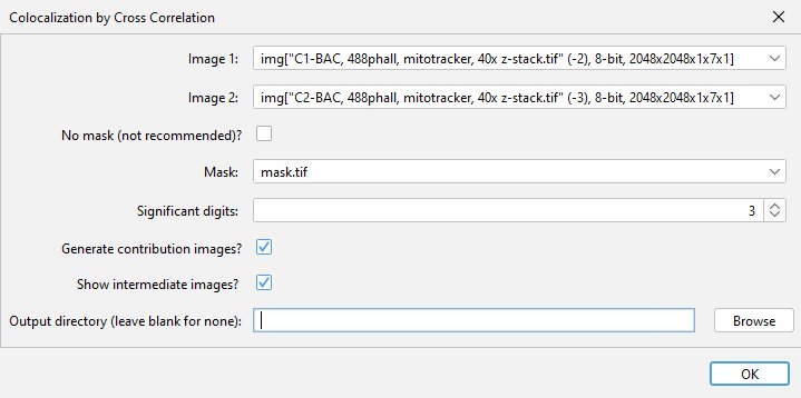 安装后,可以在 Analyze > Colocalization 菜单中找到该插件。在对话框菜单中,选择两个图像和要使用的分析掩模。如果您的染料/污点的可能定位包含整个图像,您可以选中无遮罩框。该插件还可以通过选中“生成贡献图像”复选框来计算每个输入图像中的哪些信号对结果有贡献。此进程确实使用更多内存,因此如果收到内存不足错误消息,则应禁用该进程。通过将“要拟合的高斯数”设置为 2 或更多(如下所述),可以选择将多项高斯和曲线拟合到数据。如果选中“显示中间图像”框,则插件将打开显示互相关图像的图像,在减去低空间频率分量之前和之后。这对于理解插件的功能很有用,或者如果您的样本具有偏振轴,则对于可视化相关方向很有用。有关贡献和中间图像的更多详细信息可以在下面找到。
引用 CCC
- A. McCall,(2024)互相关共定位,一种适用于超分辨率显微镜的新共定位方法。 BMC生物信息学
解释结果:
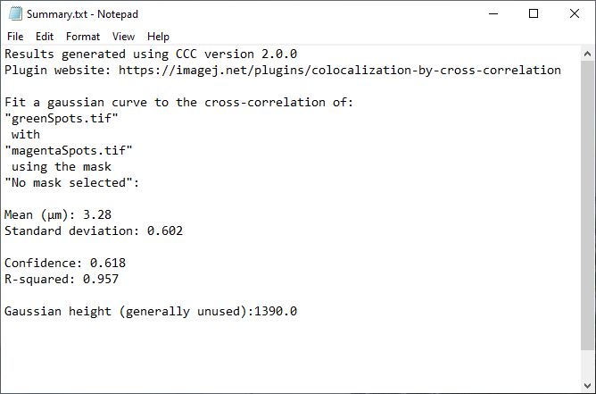
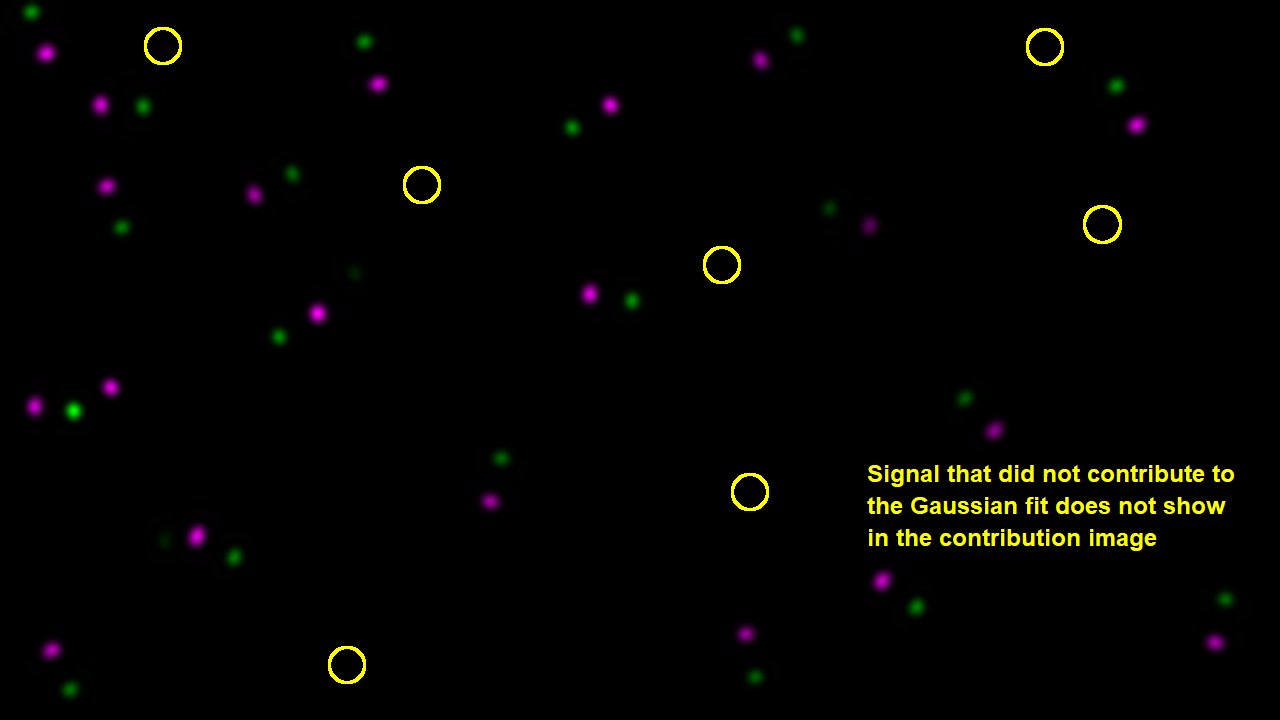
为了帮助描述结果,我们将使用如下所示的简单、理想化示例。此示例分析由相同大小的点组成的两个 2D 图像的互相关性(显示为合成图像)。这些点中的大多数都以设定的距离与其他通道的点配对,但有些点不在该距离处或未配对。从结果中我们可以看到,强相关点的间距约为 3.28 µm,标准偏差约为 0.6 µm。贡献图像突出显示彼此相关距离内的点,同时抑制该范围之外的点。在本示例中,我们使用远距离相关来突出该技术的优势之一,但这可以用于平均互相关距离接近于零的传统“共定位”图像。
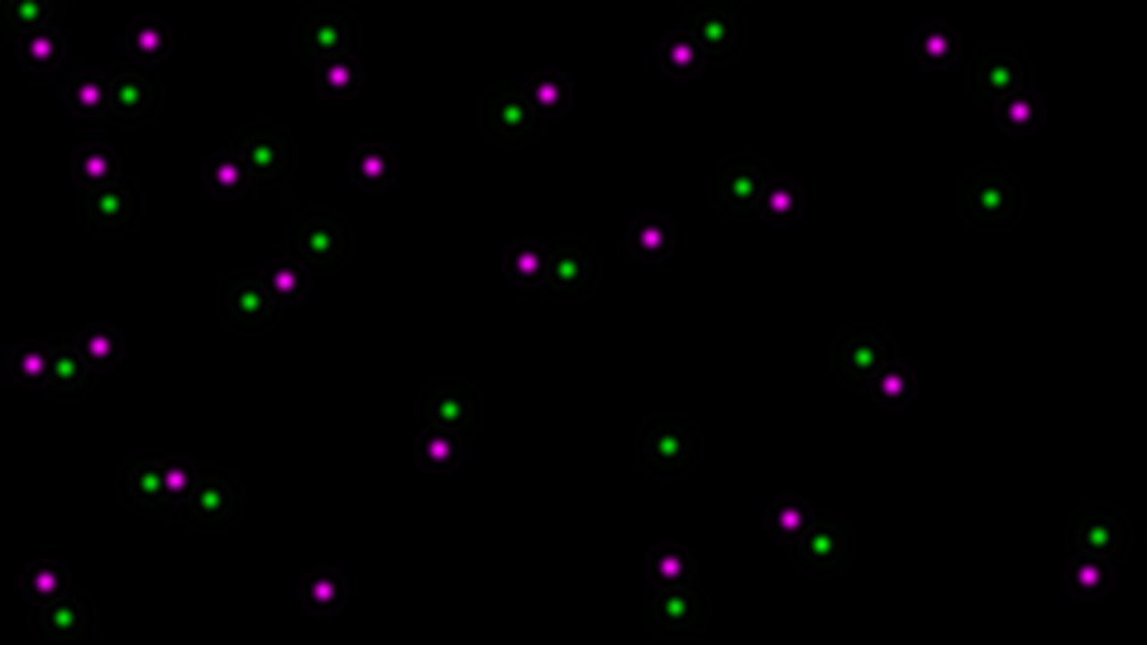 Composite of images analyzed
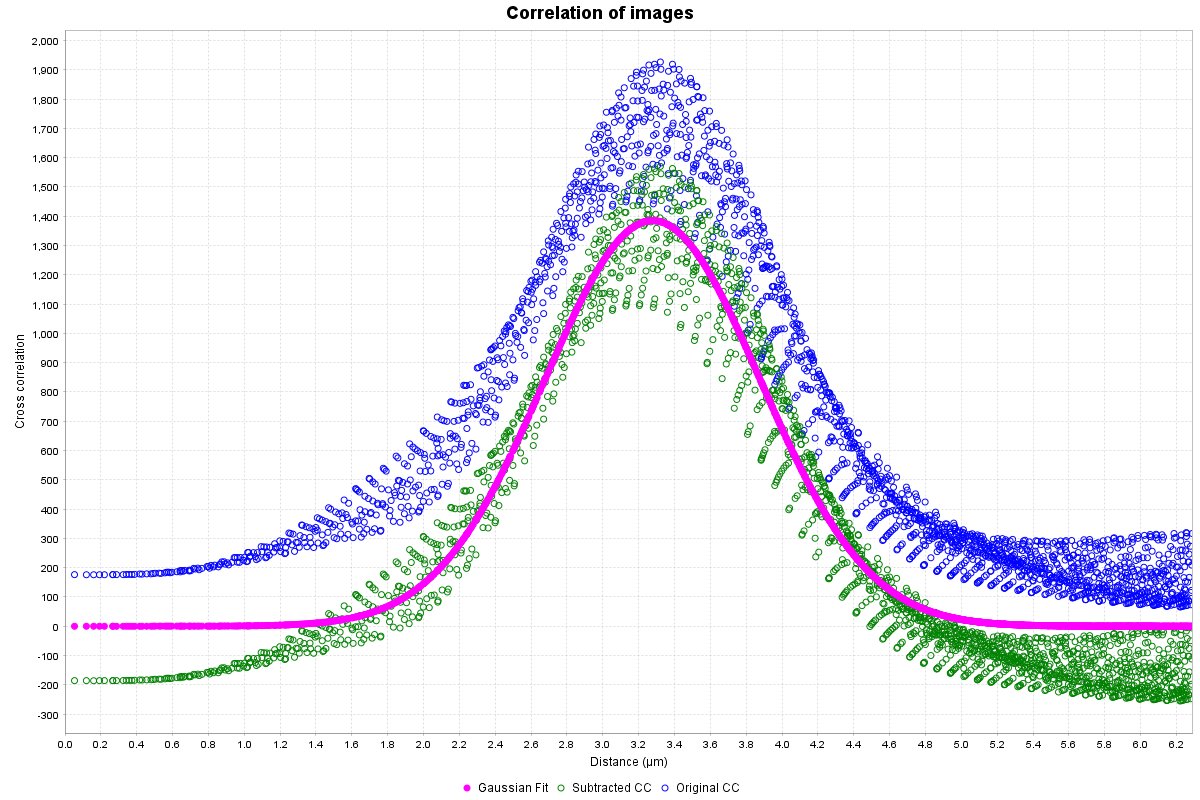 Correlogram
 Gaussian fit result
 Composit image of Gaussian fit contributions
以下是每个结果窗口的详细说明:
相关图
将显示径向剖面图,它包含原始互相关图像的径向剖面(蓝色圆圈)、减去低空间频率分量后的互相关的径向剖面(绿色圆圈)以及与减去的剖面拟合的高斯曲线(洋红色实心圆圈)。蓝色和洋红色之间的距离是下面描述的置信度值的视觉指示器。 Y 轴是互相关函数的平均值。虽然在技术上不是任意的,但它最容易被视为相对互相关的度量。图形的范围自动设置以适合高斯曲线。如果您希望查看所有数据,请右键单击该图并选择“自动范围”>“两个轴”。
高斯拟合分析
该表将包含(以缩放单位)、测量相关性的平均距离 (μ)、该相关性的标准偏差 (σ) 以及高斯拟合的峰值高度。它还包含统计度量置信度和 R 平方。下面详细解释每个参数,包括限制和改进该参数的方法。
平均值/μ
只是测量的空间相关性与高斯曲线拟合的平均距离。高斯拟合函数从未返回精确的零值,因此请确保将极小的值(例如 1.2E-17)四舍五入为零。此外,请小心解释这些零值或低于分辨率限制的任何值。在许多其他共定位方法中,只有在此范围内的空间相关性才会导致正“共定位”。对于 CCC,值为零或接近零通常意味着图像的分辨率太低,无法确定真实的平均空间相关距离,但它可能在 0 到 σ 或 2σ 范围内。您可以通过提高分辨率来更精确地测量相关距离,但这对于您的研究来说可能不是必需的。话虽这么说,从迄今为止的测试来看(并且由于 CCC 的工作原理),在某些极少数情况下,CCC 似乎确实可以返回略低于分辨率限制的准确平均值。发生这种情况是因为我们聚集了图像内的所有相关粒子。 然而,要这样解释,实验重复的结果应该是一致的。这更有可能是侥幸,而不是超分辨率的结果。
标准差/σ
测量的空间相关性的标准差。一般来说,可以通过提高输入图像分辨率来提高该值。然而,返回值也可能是由测量的空间相关性的真实变化引起的。异常高的值(例如,单个细胞图像的 σ 值约为 7-10μm)通常是由不适当的掩模或完全缺乏掩模(当掩模合理时)引起的,或者是由于一幅或两幅图像中的高分子密度的分辨率太低而引起的。
信心
置信度是 CCC 特有的一个新颖指标。它是通过将高斯拟合曲线的曲线下面积 (AUC)(在平均值 ± 3×sigma 范围内)除以原始相关径向剖面的 AUC(在相同范围内)来确定的。接近 1 的值表明真正相关的可能性很大。接近 0 的值表示两个图像之间的相关性较低甚至没有,或者需要更高的分辨率。我目前估计 ~0.10 或更大的值表示合理的相关性(在高斯曲线指定的范围内),0.2 或更大的值表示可能的真实相关性。最终,在实验重复中获得一致的结果比高于 0.2 的置信度更重要。
置信度受到许多图像质量和空间相关参数的影响,包括图像分辨率、分子密度、相关距离、不相关粒子和图像背景。一般来说,可以通过提高图像分辨率来增加低置信度值。然而,这假设存在真正的空间相关性,因为低置信度也可以简单地表明缺乏真正的相关性。如果您的信心非常低,请确保正确预处理图像并在 32 位图像上减去图像背景。
R 平方
R平方值也仅在平均值±3×sigma范围内计算,并且主要受图像中的噪声以及PSF的各向异性程度的影响。一般来说,假设信噪比合理,则无需担心 R 平方。
高斯峰高
在大多数情况下,峰值高度可能会被忽略,但它大致反映了相关性的相对强度。例如,如果您期望相关粒子的数量或相关粒子与不相关粒子的比率发生变化,但距离没有变化,则可以使用它。由于高斯曲线拟合是根据减去的互相关数据完成的,因此峰高也受到置信度等所有图像质量参数的影响。 为了使图像之间的高度具有可比性,它们必须在相同的条件下成像。重要的是,互相关结果中的值已标准化为掩模体积。因此,如果您比较高斯高度,则应考虑分析区域体积的差异。
每个图像对高斯拟合的贡献
将创建两个新图像,显示来自每个分析图像的信号,这些图像有助于互相关和高斯拟合结果。 需要注意的是,即使两个图像之间没有很强的相关性,它包含的数据始终是可见的。通常,像素强度值不应用作图像之间总体相关性的指标,但图像内的相对亮度可以用作特定信号对相关结果的贡献程度的近似指标。在上面的示例数据中可以很容易地看到这种相对亮度指示:在我们的原始数据中,所有点都具有相同的大小和强度,但是,在生成的贡献图像中,保留的点的亮度根据它们对互相关结果的贡献程度而变化(您会注意到最亮的点都朝向同一方向)。
多重高斯曲线拟合
从 v2.3.0 开始,CCC 现在原生支持将多个高斯曲线拟合为数据作为高斯和曲线。运行 CCC 时,在弹出的对话框中设置尝试拟合的高斯项数。如果两个图像之间的空间关系具有多个分量(最常见的是宽的低频分量和具有相似平均值的窄的高频分量),则多项高斯曲线会很有用。每个高斯项的置信度值是独立计算的,因此过度拟合会导致每个高斯项的置信度降低。此外,拟合过程中每增加一个高斯项都会增加额外的计算时间。
使用时间序列数据:
使用时间序列数据与使用非时间序列数据没有什么不同。数据的每一帧都会被单独分析,其方式与分析非时间序列数据的方式完全相同。因此,所有输入(包括掩码)必须具有相同数量的帧。插件生成的输出已更改,以更好地适应时间序列数据:
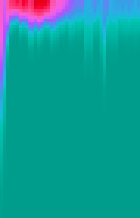
Heat map of Gaussian fit: An example of the heat map generated with time-series data, shown with the Ice lookup table. Each column of pixels shows the Gaussian curve fit to the cross-correlation for a single frame.
The most noteable difference with time-series data is how the data for the correlation plot is displayed. Instead of scatter-graphs, the plugin generates heat maps, where the x-axis is time, the y-axis is distance with 0 at the top, and the intensity is the average of the cross-correlation function at that distance. As we cannot simultaneously show the data for the three lines that would be shown in the correlation plot when using a heat map, we instead generate a three channel image. The first channel (defaults to magenta), displays the Gaussian curve fit to the profile of correlation after subtraction of random associations, equivalent to the magenta circles from the correlation plot. The second channel (defaults to green) shows the cross-correlation function results after subtraction of random associations, equivalent to the green circles from the correlation plot. And the third channel (defaults to blue) show the results of the original cross-correlation function, equivalent to the blue circle from the correlation plot.
Another change with time-series data is that in addition to the Gaussian fit analysis text window, which now displays the fit data for the frame with the highest correlation, the plugin will output a table of Gaussian fit results, showing the Gaussian fits and confidence for each frame. To save this table (if you didn’t use the auto-save feature), go to File > Export > Table…, click browse and save the file as a .csv file (you must add the extension or you will get an error message).
Lastly, the contribution images will still be generated and are functionally the same as for their non-time series counterparts. However, it’s important to note that the contribution is evaluted on a per frame basis, and thus each frame shows the signal contribution to the Gaussian fit results for that frame. Thus, if your cross-correlation distance shifts over the course of an experiment, the contribution images will display this shifting correlation.
Advantages and Disadvantages
Advantages
- High- and super-resolution compatible: Since CCC measures spatial correlation over as a function of distance, there’s no requirement for the two channels to overlap. This means that you can keep improving your resolution, and your results will generally just get better (there is a limit to this, but it would mean drastically oversampling your data).
- More details of the spatial correlation are provided, leading to a better understanding of the nature of the relation
- Image quality metrics and spatial correlation variability are built into the results (with zero effort from the user):
- Improved resolution > more accurate mean, narrower SD, higher confidence
- Higher SNR > higher R-squared
- Higher molecular density > lower confidence
- Longer spatial correlation distance > lower confidence, lower R-squared, eventually larger SD; This may seem disadvantageous, but it simply means there’s a slight bias for closer correlations, which are generally more likely to be the true correlation
- More uncorrelated particles > lower confidence, eventually causes inaccuarte mean, larger SD, and lower R-squared
Disadvantages
- The pre-processing steps are important: failure to subtract background will result in low confidence, and failure to use a mask when necessary will often result in fitting to a low spatial frequency (such as cells correlating with themselves and resulting in a mean of 0, and a SD of 5-10 µm)
- Results are sensitive to mask selection: changes to the mask can cause significant changes to the results. If very slight mask changes cause significant changes to the results it likely means you are right on the border of the required resolution for the spatial correlation you are measuring, and you should try to improve your resolution
- The plugin uses a lot of memory, more than I ever thought it would, and nearly all the memory used scales with image size. I’ve tried reducing the memory requirement as much as I can, but it still uses a ton. Changing the input image bit-depth makes almost no difference, as all the calculations and data generated are 32-bit. However, there are some things you can do:
- Crop or split the image. If you’re studying correlations inside a cell, you could analyze each cell individually. I don’t recommend cutting across a mask though, this will change your results.
- Turn off intermediate images and contribution images. Both of these add a significant amount to the total memory required for the plugin.
- Buy more RAM. It’s not that expensive, and it’s usually super easy to install. This may not be an option if you use a Mac though.
- Run the analysis with a cloud computing service. CCC was made using SciJava and is Headless mode compatible, making it possible to run the analysis remotely.
How it works & intermediate images description:
First, this plugin applies the provided mask to both images, setting any pixels outside the masked region to zero. If this were not done, these pixels would contribute to the original cross-correlation result, but this contribution would then always subtracted out during the process described below, leading to a decrease in confidence. After applying the mask, this plugin then performs an initial cross-correlation to create a original cross-correlation image. Bright regions in the cross-correlation image correspond to a high correlation between the images when the second image is shifted by a vector equal to the distance form the center of the cross-correlation image to the bright region. Thus, if you see a bright spot in the cross-correlation image that is 2 µm to the left of the image center, it means their is a positive correlation between image 1 and image2 when image2 is shited left 2 µm.
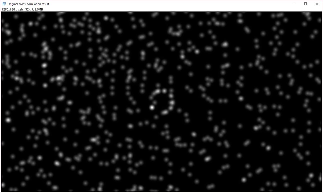 Initial, unmodified cross-correlation result
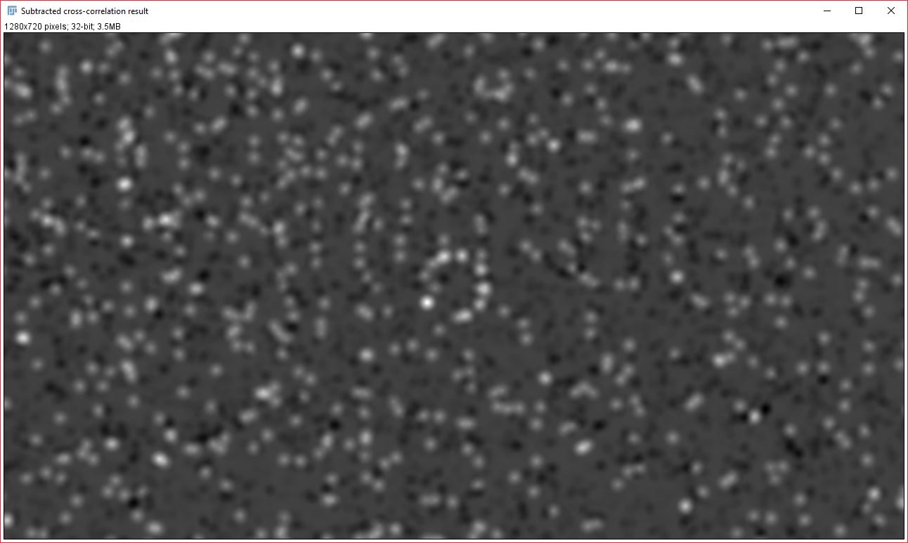 Cross-correlation result after subtraction of low frequency component
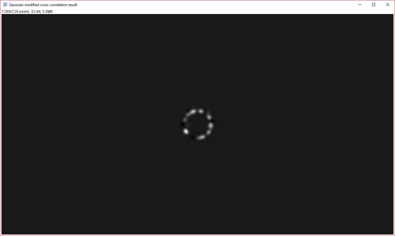 Gaussian-fit modified cross-correlation
为了消除低空间频率结构/数据(例如细胞和细胞核)的贡献,然后从原始相关图像中减去从低空间频率图像生成的第二互相关图像。对于此过程,计算掩模内第一个输入图像的所有像素的平均强度,然后创建一个新图像,其中掩模内的所有像素都设置为该平均值。该图像是第一个输入图像的平均低空间频率图像。然后将该低频图像与第二输入图像进行互相关,并且所得到的互相关图像是低频分量,从原始互相关图像中减去该低频分量。掩模下均值过程仅应用于一幅图像,因为将其应用于两幅图像不会导致结果出现显着差异,并且会使用更多的时间和内存。然后,我们生成减去数据的径向轮廓并对其拟合高斯曲线。我们还在减法之前生成原始相关数据的径向剖面,因为这是建立置信度度量所必需的。置信度计算为减去的相关径向分布(在平均值±3×sigma范围内)的曲线下面积(AUC)除以原始相关径向分布(在相同范围内)的AUC。置信度值以及高斯拟合的平均值和西格玛显示在日志窗口中。置信度值越高,越接近 1,表明两幅图像在指定距离处可能具有真实的空间相关性。
为了生成贡献图像,我们通过有效地将减法互相关图像与高斯拟合相乘来进一步修改减法互相关图像,以创建仅保留高斯曲线范围内的数据的互相关图像。然后使用该高斯修改的互相关图像来反计算贡献图像。 Image1Contribution = (image2 * gaussModifiedCorr) × image1。 Image2Contribution = (image1 ★ gaussModifiedCorr) × image2。关键:* -> 卷积,★ -> 关联。
替代命令
这些命令可以通过 CCC 在“分析”>“共定位”>“通过互相关进行共定位”下找到。仅当原始 CCC 由于内存不足(并且没有更高内存的计算机可用)而失败,或者您出于共定位以外的目的生成互相关数据时,才建议使用这些数据。
CCC - 没有信心
CCC的无置信度命令与上述原始命令非常相似,但它不计算原始互相关。相反,它能够在第一次互相关之前消除低频贡献并生成减去的互相关结果,而无需生成原始结果。这样做的缺点是现在无法计算置信度值,因为这需要原始的互相关数据。无置信度版本不适用于生成低置信度结果的数据。这仅适用于由于内存限制而无法由原始 CCC 处理的非常大的数据集。即使在这些情况下,最佳实践也是获取原始数据集的裁剪区域并执行 CCC 以获得数据集置信值的近似值。
请注意:对于延时数据,由于无法使用置信度来评估“最佳”帧,因此使用标准偏差最小的帧。因此,CCC 的原始版本和无置信版本之间的最佳框架可能存在显着差异。
只是互相关
“Just Cross Correlation” 该命令简单地对两个输入图像进行互相关,并计算径向轮廓。不计算高斯曲线拟合或统计数据。如果 CCC 和 CCC - No Confidence 由于内存不足而失败,则可以仅使用互相关,这样您至少可以看到一条互相关曲线,或者它可以用于非高斯关系,例如下面描述的关系。
我最初做这个是因为有人想通过 microCT 扫描确定关节的平均厚度。关节两侧两个骨骼的仅边缘版本的互相关生成了一条 S 曲线(在峰值后下降,但对于高斯拟合来说速度太慢),之后他们可以提取曲线数据并使用单独的应用程序对其拟合 S 曲线。
主要修改
v2.3 中的新结果表顺序
结果表中的参数顺序已更改,以适应多重高斯拟合。这种顺序更改可能会影响自动从此输出表读取的脚本结果。顺序从 {均值、SD、置信度、R 平方、高度} 更改为 {<Mean, SD, Height, Confidence>(按高斯)、R 平方}。
v2.3 中新的置信度值计算
随着 v2.3 中多高斯拟合的发布,置信度计算更改为使用高斯拟合曲线的曲线下面积 (AUC) 代替减去的相关图数据。对此进行了更改,以便多高斯拟合的每个单独的高斯都有自己的置信值。
v2.1 中的结果略有不同
在 CCC v2.1 中,从互相关中删除数据低频分量的方式已更改,以允许创建“不置信度”命令。基本上,不是将图像 1(具有平均值图像的掩模)的低频分量与图像 2 进行互相关,如上面工作原理部分所述,在 v2.1 中,在与图像 2 互相关之前,从图像 1 的掩模边界内的每个像素中减去掩模内的平均像素值。这有效地在执行互相关之前而不是之后减去低频分量。在测试期间,此过程生成与上述版本 2 方法相同或非常相似的结果。我相信它并不总是相同的原因是由于舍入的差异,因为新的 v2.1 方法跳过了 v2 的几个舍入步骤。我对“无置信度”命令和原始 CCC 命令都进行了此更改,因为我希望它们产生相同的结果,并且因为此方法的内存效率更高。
我不会更改上面对“它是如何工作的”的描述,因为我觉得这更容易理解,而且结果实际上是相同的。
删除像素随机化
在 CCC v2 中,重复像素随机化过程(如 BMC 生物信息学出版物中所述)被掩模方法内的平均值取代,以去除低空间频率分量。这个新过程速度更快、内存效率更高,并且允许 CCC 在提供相同输入时生成一致的结果。虽然表面上看起来很不同,但如果 v1 使用无限重复,这实际上是相同的过程,并且会产生相同的结果。这最终是因为互相关不必在每次随机化之后进行,总体结果在重复之间进行平均,而是可以首先重复图像的随机化并平均,然后将所得图像与第二个图像进行互相关。有效地:
\[\lim\limits_{n \to \infty} \left(\frac{\sum_{i=1}^n \left(rand(Img1)_i \star Img2\right)}{n}\right) = \lim\limits_{n \to \infty} \left(\left(\frac{\sum_{i=1}^n \left(rand(Img1)_i\right)}{n} \right)\star Img2\右)\]无限次随机化和平均图像的过程将产生仅具有平均强度值的图像。因此,为什么使用掩模下的平均强度。