



自迁移出 MediaWiki 以来,本页内容尚未经过审查。如果您愿意帮忙,请查看帮助指南!
2D 和 3D 衍生分析图像。对于 ImageJ 1.x 插件,请参阅this page。
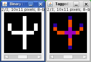 Example of voxel classification
|
一般说明
Example of voxel classification
This plugin tags all pixel/voxels in a skeleton image and then counts all its junctions, triple and quadruple points and branches, and measures their average and maximum length. The tags are shown in a new window displaying every tag in a different color. You can find it under Analyze › Skeleton › Analyze Skeleton (2D/3D). See Skeletonize3D for an example of how to produce skeleton images.
体素根据其26个邻居分为三个不同的类别:
- 终点体素:如果他们的邻居少2个。
- 连接体素:如果它们有超过2个邻居。
- 板体素:如果它们正好有2个邻居。
端点体素以蓝色显示,平板体素以橙色显示,连接体素以紫色显示。
请注意,按照这种表示法,连接体素的数量可能与实际连接体素的数量不同,因为某些连接体素可以不相同。
主要选项
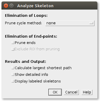 Main dialog of the AnalyzeSkeleton plugin
In the main dialog of the plugin the user can select some options to
- 修剪构造中可以进行循环(通过选择一种修剪循环方法)。
- ** 修剪以端点结束的任何端点**(通过检查“修剪结束”),如 BoneJ 中的 Michael Doube 实施所。
- In this case, if a ROI was selected in the input image, another option is enabled: Exclude ROI from pruning. If selected, pruning will not be applied to end-points contained by the ROI. An application of this feature is described in Strahler Analysis.
- 使用“Depth-First Search”计算每个餐具的最大最短路径。在这种情况下,最短路径将显示在一个新闻中,其中包含白色的餐具和洋红色的最短路径。由 Huub Hovens 实施。
- ** 显示有关图像中每个重构的分支的详细信息**。
- ** 显示标记的配件**。将显示一个额外的图像输出,其中包含带有相应 ID 的每个配件的配件标签。
循环检测和剪枝
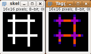 Example of cycle detection and pruning
Since the 2009/09/02 version of the code, the possible cycles or loops in the skeleton can be detected and pruned previous to the analysis. In this sense, the initial plugin dialog offers 4 options:
- 无:不执行循环检测或修剪。
- 最短分支:循环分支中最短的分支将在其中点被切断。
- 最低强度体素:循环体素中最暗的体素将在输入图像中被剪切(设置为0)。
- 最低强度分支:循环分支中最暗(平均)的分支将在其最暗的体素中被切割。
对于最后两个方法,将弹出另一个对话框,要求用户在打开的图像中选择原始(灰度)图像以执行强度计算。基于重构中的经典APSP (all pairs shortest path)(DFS)进行循环检测。重构被视为tortuosity,其中端点和交汇处为节点,板分支为边。在以DFS方式访问图时,指向未访问节点的边/分支被标记为TREE边,而指向已访问节点的边被标记为BACK边,这涉及到循环的存在的边缘。分类后,BACK边缘会紧邻其前一个边缘回溯,以计算属于每个循环的所有边缘并继续进行剪枝。
这种方法唯一已知的限制是存在唤醒循环。在这些情况下,对插件的第二次调用通常足以消除所有剩余的循环。
结果表
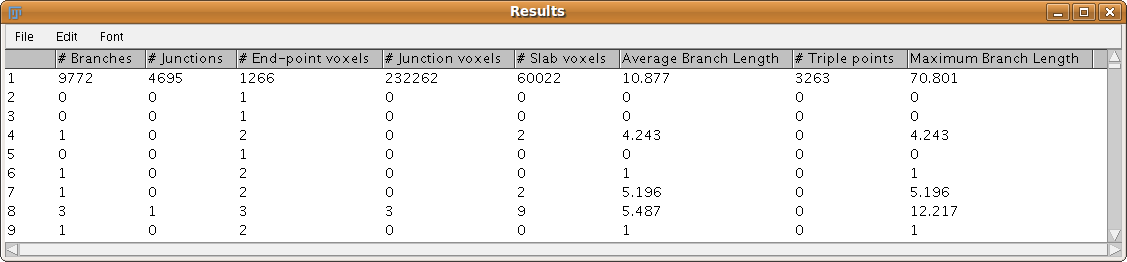 Example of AnalyzeSkeleton Results table
After classification, a “Results” window is displayed showing for each skeleton in the image:
- 分支(板段,通常连接端点、端点和交汇点或交汇点和交汇点)的数量。这里还考虑了圆形支架的特殊情况。
- 端点类型的体素数量:端点、平板和连接体素。
- 具有任意数量的投影分支的实际连接点(合并互连连接点体素)的数量。
- 三重点(恰好有 3 个分支的交汇点)和四重点(4 个分支)的数量。
- 分支的平均和最大长度,以相应的单位表示。
AnalysisSkeleton 能够在一张图像中处理最多231-1 个重构(仅受java Integer.MAX_VALUE限制)。
####详细信息
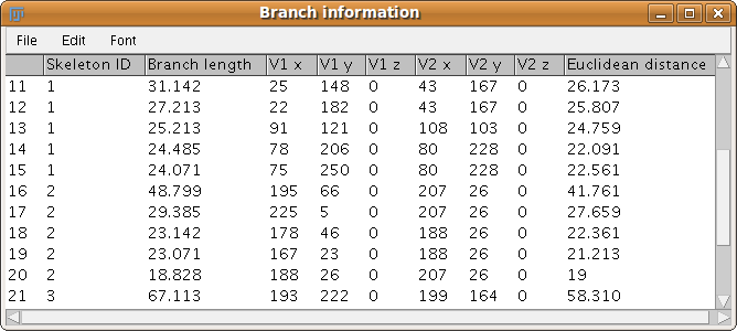 Example of AnalyzeSkeleton Branch information window
When calling the plugin, if the “Show detailed information” checkbox is marked, a complementary results table called “Branch information” is shown.
在这里表中,我们显示所有的中继信息:
- 骨架ID,
- 规划的分支长度,
- 端点端点的3D坐标(所谓的V1和V2端点),
- 这些极值点之间的欧几里得距离。事实证明,该值可以很好地指示 3D 对象的 undirected graph。
分支按长度递减排序。
视频教程
快速了解 Skeletonize3D 和 AnalyzeSkeleton 实际以及应用示例,您可以查看此video tutorial。
本教程逐步介绍了如何:
- 切除3D图像以提取相关形态信息
- removing the noise
- and binarizing
- 使用Skeletonize3D提取二值图像的重构
- 使用AnalyzeSkeleton分析3D图像中生成的重建
可视化
使用3D_Viewer库,我们可以轻松显示重构和分析结果:
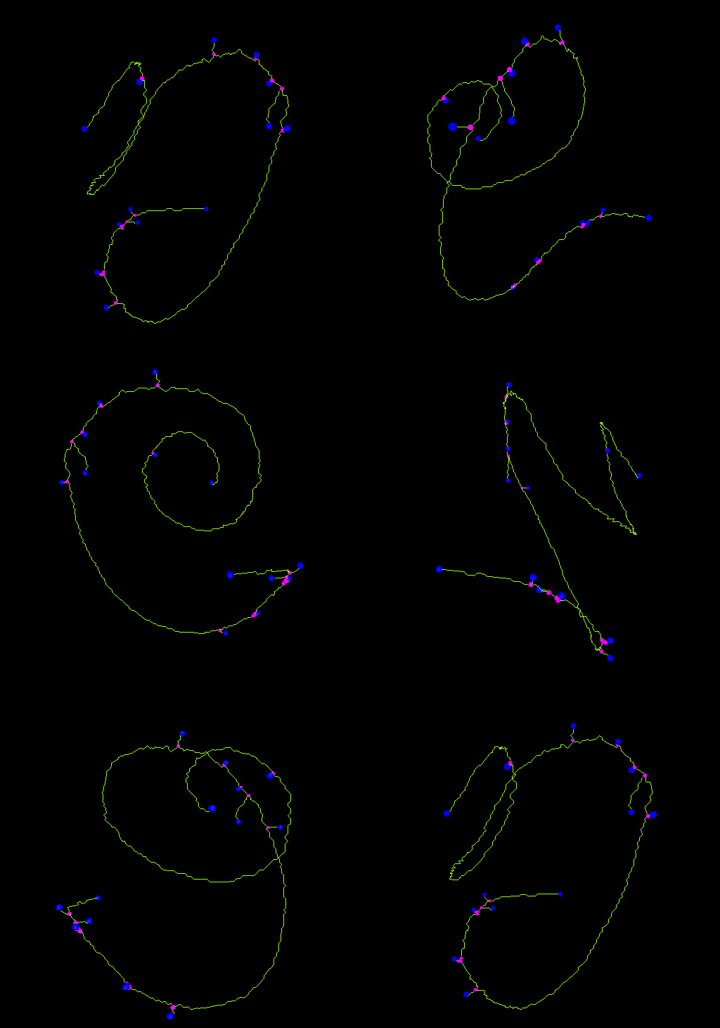 3D skeleton of bat cochlea volume rendered in the viewer after voxel classification
|
 Smooth (by 3D Gaussian filter) bat cochlea volume rendered in the viewer
|
 Bat cochlea volume rendered in the viewer with its corresponding classified skeleton
|
编写分析骨架脚本
还可以从脚本调用AnalyzeSkeleton功能,利用其库方法或以静默模式执行整个分析。
从脚本中使用静默模式
您可以从脚本中使用AnalyzeSkeleton,而不显示任何结果。如果您想在脚本中使用结果而不会让用户因大量弹出的结果而感到烦恼,那么这非常有用。
这是 JavaScript 中的一个示例: importPackage(Packages.ij); importPackage(Packages.sc.fiji.analyzeSkeleton);
// Takes a binary image as input
var imp = IJ.getImage(); // get current open image

// Skeletonize the image
IJ.run(imp, "Skeletonize (2D/3D)", "");

// Initialize AnalyzeSkeleton_
var skel = new AnalyzeSkeleton_();
skel.calculateShortestPath = true;
skel.setup("", imp);

// Perform analysis in silent mode
// (work on a copy of the ImagePlus if you don't want it displayed)
// run(int pruneIndex, boolean pruneEnds, boolean shortPath, ImagePlus origIP, boolean silent, boolean verbose)
var skelResult = skel.run(AnalyzeSkeleton_.NONE, false, true, null, true, false);

// Read the results
var shortestPaths = skelResult.getShortestPathList().toArray();
var branchLengths = skelResult.getAverageBranchLength();
var branchNumbers = skelResult.getBranches();

var totalLength = 0;
for (var i = 0; i < branchNumbers.length; i++) {
    totalLength += branchNumbers[i] * branchLengths[i];
}

var cumulativeLengthOfShortestPaths = 0;
for (var i = 0; i < shortestPaths.length; i++) {
    cumulativeLengthOfShortestPaths += Number(shortestPaths[i]);
}

// Use the readout within the script
IJ.log(totalLength);
IJ.log(cumulativeLengthOfShortestPaths); ###按长度树枝
以下 Beanshell 脚本会缩减输入的分支(如果它们低于特定长度): // @ImagePlus(label=”Skeleton image”, description=”Binary image skeletonized with Skeletonize3D”) image // @double(label=”Length threshold”, description=”Minimum branch length to keep”) threshold // @OUTPUT ImagePlus prunedImage
import sc.fiji.analyzeSkeleton.AnalyzeSkeleton_;
import sc.fiji.analyzeSkeleton.Edge;
import sc.fiji.analyzeSkeleton.Point;
import ij.IJ;

// analyze skeleton
skel = new AnalyzeSkeleton_();
skel.setup("", image);
skelResult = skel.run(AnalyzeSkeleton_.NONE, false, false, null, true, false);

// create copy of input image
prunedImage = image.duplicate();
outStack = prunedImage.getStack();

// get graphs (one per skeleton in the image)
graph = skelResult.getGraph();

// list of end-points
endPoints = skelResult.getListOfEndPoints();

for( i = 0 ; i < graph.length; i++ )
{
    listEdges = graph[i].getEdges();

    // go through all branches and remove branches under threshold
    // in duplicate image
    for( Edge e : listEdges )
    {
        p = e.getV1().getPoints();
        v1End = endPoints.contains( p.get(0) );
        p2 = e.getV2().getPoints();
        v2End = endPoints.contains( p2.get(0) );
        // if any of the vertices is end-point
        if( v1End || v2End )
        {
            if( e.getLength() < threshold )
            {
                if( v1End )
                    outStack.setVoxel( p.get(0).x, p.get(0).y, p.get(0).z, 0 );
                if( v2End )
                    outStack.setVoxel( p2.get(0).x, p2.get(0).y, p2.get(0).z, 0 );
                for( Point p : e.getSlabs() )
                    outStack.setVoxel( p.x, p.y, p.z, 0 );
            }
        }
    }
}

prunedImage.setTitle( image.getShortTitle() + "-pruned" ); 请注意,由于删除了端点和板而不是交汇点,可能会创建小分支(以防止破坏某个值的分支)。因此,您可能需要运行该脚本几次才能删除所有不需要的分支。
在 3D 查看器中可视化工件
以下 Beanshell 脚本显示了 3D 查看器中的体素分类: // @ImagePlus(label=”Skeleton image”, description=”Binary image skeletonized with Skeletonize3D”) image
import sc.fiji.analyzeSkeleton.AnalyzeSkeleton_;
import sc.fiji.analyzeSkeleton.Edge;
import sc.fiji.analyzeSkeleton.Point;
import ij.IJ;
import ij3d.Image3DUniverse;
import org.scijava.vecmath.Point3f;
import org.scijava.vecmath.Color3f;

// analyze skeleton
skel = new AnalyzeSkeleton_();
skel.setup("", image);
skelResult = skel.run(AnalyzeSkeleton_.NONE, false, false, null, true, false);

// get calibration
pixelWidth = image.getCalibration().pixelWidth;
pixelHeight = image.getCalibration().pixelHeight;
pixelDepth = image.getCalibration().pixelDepth;

// get graphs (one per skeleton in the image)
graph = skelResult.getGraph();

// create 3d universe
univ = new Image3DUniverse();
univ.show();

// list of end-points
endPoints = skelResult.getListOfEndPoints();
// store their positions in a list
endPointList = new ArrayList();
for( Point p : endPoints )
    endPointList.add( new Point3f(
        (float)( p.x * pixelDepth ),
        (float)( p.y * pixelHeight ),
        (float)( p.z * pixelDepth ) ) );
// add end-points to the universe as blue spheres
univ.addIcospheres( endPointList, new Color3f( Color.BLUE ), 2, 1f, "End-points");

// list of junction voxels
junctions = skelResult.getListOfJunctionVoxels();
// store their positions in a list
junctionList = new ArrayList();
for( Point p : junctions )
    junctionList.add( new Point3f(
        (float)( p.x * pixelDepth ),
        (float)( p.y * pixelHeight ),
        (float)( p.z * pixelDepth ) ) );
// add junction voxels to the universe as magenta spheres
univ.addIcospheres( junctionList, new Color3f( Color.MAGENTA ), 2, 1f, "Junctions");

for( i = 0 ; i < graph.length; i++ )
{
    listEdges = graph[i].getEdges();

    // go through all branches and add slab voxels
    // as orange lines in the 3D universe
    j=0;
    for( Edge e : listEdges )
    {
        branchPointList = new ArrayList();
        for( Point p : e.getSlabs() )
            branchPointList.add( new Point3f(
                (float)( p.x * pixelDepth ),
                (float)( p.y * pixelHeight ),
                (float)( p.z * pixelDepth ) ) );
        // add slab voxels to the universe as orange lines
        univ.addLineMesh( branchPointList, new Color3f( Color.ORANGE ), "Branch-"+i+"-"+j, true );
        j++;
    }
} ## API文档
代码的最新文档可以在这里找到:
http://javadoc.imagej.net/Fiji/sc/fiji/analyzeSkeleton/package-summary.html
变更日志
所有变更护士在GitHub source repository中查看。
2010/12/28:Jan Eglinger 添加了在静默模式下由脚本调用的插件的代码。
2010/09/27:添加了 Huub Hovens 的代码来检测每个重构中的最短最大路径,并添加了 Michael Doube 的代码来尖端以端点末端的分支。
2010/08/26:修复了以下错误:如果分支终止于已访问的交汇点,则从端点访问树时会向边缘分配错误的最终端点(V2)。彼得·C·马克斯报道。
2010/01/12:感谢Peter Marks,修复了从路口开始时正确访问树木的错误(它们没有被添加到重新访问列表中,有时导致一些树木被分割)。
2009/12/04:添加四点计算。
2009/09/13:删除了日志窗口并创建了详细信息选项和分支信息表。
2009/09/02:增加了检测和修剪周期的功能。
2009/08/10:修复了处理单体圆柱形的特殊情况的小错误。
2009/08/06:修复了2个错误:计算结点之间的分支和圆形树中的平板体素数量。
2009/08/05:修复了减慢实际路口数量计算速度的错误。
2009/06/19:修复了一些计算中的错误,将分支数量从 255 个增加到 2¹⁵-1,并添加了新的(之前未处理的)案例。
2009/04/07:为图像中的每个部件添加了不同的计算,并在日志窗口中添加了一些额外信息。
2009/03/05:添加最大分支长度计算。
2008/11/19:添加了三个重点计算并修复了错误,居民修改原始图像并在输出图像中保留其结构。
2008/11/16:首次发布。
参考文献和引用
如果您需要引用该插件,请引用以下论文:
最短路径计算其应用已发表为:
- G. Polder、H.L.E Hovens 和 A.J Zweers,使用图形分析测量水下水生植物的芽长 (2010),参见:ImageJ 用户和开发者会议记录,Recherche Public Henri Tudor 中心,卢森堡,10 月 27-29 日,第 172-177 页。
AnalyzeSkeleton也是BoneJ的一部分,ImageJ中用于分区图像分析的插件:
- Michael Doube、Michal M. Klosowski、Ignacio Arganda-Carreras、Fabrice P. Cordelieres、Robert P. Dougherty、Jonathan S. Jackson、Benjamin Schmid、John R. Hutchinson、Sandra J. Shefelbine,BoneJ: Free and extensible bone image analysis in ImageJ,《Bone》,第 47 卷,第 6 期,2010 年 12 月,第1076-1079页。
许可证
该程序是免费软件;您可以根据自由软件基金会 (http://www.gnu.org/licenses/gpl.txt) 发布的 GNU 通用公共许可证 的条款重新分发和/或修改它。
分发此程序的目的是希望它有用,但不提供任何保证;甚至没有适用性或特定用途适用性的默许保证。有关更多详细信息,请参阅 GNU 通用公共许可证。