


SpotSpine
该插件允许检测和统计树突棘,分割脊柱,追踪脊柱,询问定量形态测量。
脊柱检测和脊柱头部分割使用插件3D ImageJ Suite中的算法。
脊柱颈部追踪使用插件SNT中的算法。
作者
让-弗朗索瓦·吉尔斯, 托马斯·布迪埃, 蒂亚戈·费雷拉, 尼古拉斯·赫克。
文档
运行 SpotSpine 之前需要执行步骤
在使用SpotSpine之前,应跟踪树突,并将跟踪的模型保存为swc文件格式。 有一些软件可以追踪树突,例如 ImageJ 插件 SNT、NeuTube、Neuronstudio 等。 其他格式可以转换为SWC。
运行 SpotSpine 之前,将图像堆栈和包含树突模型的 .swc 文件放在同一文件夹中。SWC 文件的名称应与图像堆栈的名称完全相同。您可以将多个图像和包含树突模型的 .swc 文件放在同一个文件夹中;SpotSpine 会自动读取图片名称并找到对应的 swc 文件。
建议提高图像堆栈的信噪比。一般建议相反,但去噪就可以了;插件PureDenoise提供了非常高的效率。
使用 SpotSpine
1. 打开图像堆栈
如果不是,则应设定图像。转到“图像”>“属性”并给出像素宽度、像素高度、体素深度(即图像堆栈的z步长)(以微米为单位)。
启动 SpotSpine:插件>Spot Spine
2. 选择脊柱检测参数的值
通过发现刺的局部顶点来检测刺。局部顶点是邻近体素强度的体素。将在每个脊柱头部检测到最高强度的体素。尽管如此,仍然需要调整一些参数重低音、脊柱或树突表面出现局部顶点。请注意,在树突模型覆盖的体素中无法检测到顶点。
可以调整三个参数,但您可以在下一步中再次更改这些设置(请参阅第 4 节)。
1.阈值强度 Determine that value by estimating the intensity of the spine head that is the less bright in the image. The threshold value means that any maxima which intensity is below that value will not be detected. If the value is too high, some spines will be missing. If the value is too low, some maxima may be detected in the background.
- 到枝晶的最小距离和到枝晶的最大距离 Estimate the minimal and maximal distance from the border of the dendrite. Without a mimimum distance, some maxima may be detected within the dendrite if the swc model does not cover the whole dendritic diameter. With a too high value for the maximum distance, some maxima may be detected in a neighbouring dendrite. 3.点击“确定”导入树突模型并检测树突刺
树突模型已导入图像中(但在该步骤中不可见)。
在树突模型所关注的体积内无法检测到峰值。 检测到图像堆栈的顶部和最大投影上的绿色显示。
您可以修改亮度和支撑(图像>调整>亮度/支撑),可以放大和缩小(缩放图标,或向上和向下箭头),可以在缩放图像内移动(手形图标)。
用户界面上的Change LUTs将使树从蓝色变为灰色。您可以进一步更改每个通道的颜色(图像>查找表)。
4.编辑脊柱检测结果
!如果在一个脊柱头部检测到多个局部顶峰,则令它们全部保留。如果只保留一个,那么就只分割脊柱头部的一部分。请参见调音功能第6节。
目标是在所有脊柱头中都具有局部顶点,但在其他地方都没有。因此,可以调整一些参数,并且可以进行手动编辑。不过,如果保留了错误的顶点,则可以在下一步中删除错误的脊柱;如果某个脊椎没有顶点,则可以在下一步中添加该脊椎(请参见第6节)。
可以调整以下参数:
- 最大本地内核大小:
Expand/ReduceThis parameter corresponds to the control of the minimal distance imposed between each local maxima, enabling to adapt to either sparse or dense spine density along the dendrite. - 到树突边界的距离 Minimum and maximum distances from the border of the dendrite, in between which the maxima are detected. It is the same parameter as in Section 2.
- 强度 Mimum intensity value a local maximum should have to be detected. It is the same parameter as in Section 2. The local maxima removed by adjusting the above parameters become red.
- 手动编辑 It is possible to manually add or delete local maxima. Add a new maximum : Shift+left click Delete a maximum: Alt+left click 无需精确单击意象的体素,只需单击旁边的即可。 图像堆栈和最大投影是同步的,因此可以通过单击最大投影图像来删除或添加图像堆栈中的局部顶点。
5.单击“确定”以分割脊柱头
正文的脊柱头部显示在图像堆栈中,最大投影为红色。
每个脊柱头都有一个与标签相对应的强度值,编号从 1 到 n。,有些脊柱可能头部不太明显。为确保所有脊柱头部可视化:因此图像调整>亮度/按键“设置”最小显示值=0 最大显示值=1。
您可以修改亮度和支撑(图像>调整>亮度/支撑),可以放大和缩小(缩放图标,或向上和向下箭头),可以在缩放图像内移动(手形图标)。
用户界面上的Change LUTs将使树从绿色变为灰色。您可以进一步更改每个通道的颜色(图像>查找表)。
6。编辑脊柱头部分割的结果
-
分割参数的调整 Unclick automatic if you wish to modify the parameters for segmentation. After the parameters have been modified, click on Update.
The distribution of the intensity around each local maximum is analyzed to determine the border of the spine head. “Radius” is the size of the 3D region analyzed around the local maximum. “SD value” will influence the size of the segmented spine heads. A value of 2 retrieves bigger spine heas, a value of 1 retrieves smaller spine heads. Depending on the input image, the difference may be minimal or substancial. “Gauss” performs a gaussian fit of the intensity distribution to determine the intensity value of the border of the spine head. “Mean” is another way to determine the intensity value of the border of the spine head, for this a “Weight” value should be set. The intensity is determined for each spine independently, but “Constant” allows to set a single intensity value for the border of all spine heads. After the intensity value of the border of the spine head has been computed, the algorithm starts from the local maximum to iteratively fill the spine head. There are three variations for the iterative process : Classical, Maximum, Block. You may give a try if Block does not give satisfactory results.
This « Spot Sgmentation » process is described at this page with a tutorial available as pdf and in the Figure 1 of the publication.
- 脊椎头部的手动版本**
Both images are synchronized so when clicking in the maximum projection, the object is selected by the analysis of the 3D content of the image stack within a region centered around the 2D coordinates of the mouse location.
For the purpose of merging, and delete several spine heads, the selection is cumulative. Therefore, you should click again on a spine head if you wish to unselect it.
Add: click in the image to define a region of interest, the plugin will detect a local maximum and segment the objectDelete: click on a spine head to select it and then deleteMerge: when more than one local maxima are found in one spine, the spine head is made of more that one object. Select all the objects corresponding to that spine head, then Merge. Can be required especially for large spines in which more than one maximum is found.Dilate: click on a spine head to select it and then increase its sizeErode: click on a spine head to select it and then decrease its size 7.选择一个选项来分析颈椎
-
Finish– 不要震动颈部 This will skip the analysis of the spine necks. It applies if the necks are simply not visible in the image, which can happen for example with GFP labeled dendrite, when the amount of GFP in the neck is too low to be detected.You can save the image stacks that is a composite with your image and the segmented spine heads.
In the log window, the following informations are given : Image file name, dendrite length in microns, number of spines.
A ResultTable is displayed, that is explained in Section 8. Each spine has a label given in the ResultTable; each spine head in the image has an intensity equal to label number.
-
Straight– 从脊柱头到树突画直线 This will trace straigth lines from each spine heads to the border of the dendrite. It applies when the necks are not visible in the image, and an estimate of the spine length is wanted.A composite image stack is displayed, that contains the following channels : 1st channel = Spine heads 2nd channel = Straight lines from spine head border to dendrite border 3rd channel = Dendrite model 4th channel = Image stack You can save the image as a composite. You can split the channels (Image>Color>Split channels)
In the log window, the following informations are given : Image file name, dendrite length in microns, number of spines.
A ResultTable is displayed, that is explained in Section 8. Each spine has a label given in the table. But spines in the images have different intensities to improve their visibility using muticolor rendering. And the spine necks have other colors. For Spines labeled 1, 2, 3…Spine heads are labeled 10, 20, 30…and their necks 15, 25, 35… In addition to multi-color rendering, this code allows to specifically select spine heads and spine necks with the 3D ROIManager or with macros using the plugin 3DImageSuite.
-
Next– 颈部凹陷 This will trace spine necks using algorithm from the SNT plugin.A composite image stack is displayed, that contains the following channels: 1st channel = Spine heads 2nd channel = Straight lines from spine head border to dendrite border 3rd channel = Dendrite model 4th channel = Image stack You can save the image as a composite. You can split the channels (Image>Color>Split channels).
In the log window, the following informations are given : Image file name, dendrite length in microns, number of spines.
A ResultTable is displayed, that is explained in Section 8. Each spine has a label given in the table. But spines in the images have different intensities to improve their visibility using muticolor rendering. And the spine necks have other colors. For Spines labeled 1, 2, 3…Spine heads are labeled 10, 20, 30…and their necks 15, 25, 35… In addition to multi-color rendering, this code allows to specifically select spine heads and spine necks with the 3D ROIManager or with macros using 3DImageSuite.
Manual editing of the spine necks Delete a neck path : With the first channel of the image composite active, click in one spine head to select it, click on « Delete path ». The neck is deleted.
Create a new path : With the first channel of the image composite active, shift+click in the image next to the location that will be the starting point of the path, click on « Update path ». A new neck path is created.
The ResultTable is automatically updated.
Finishends the whole process 8.了解结果表
可以使用 SpotSpine 选项选择测量参数
结果表可以保存为 .csv 文件(在表中:菜单 > 保存)。如果保存为 Excel 文件,请注意各列之间以逗号分隔。
测量以下参数:
| 参数 | 描述 |
|---|---|
| 铌 | 表中的行号(请注意第一个值=0) |
| 名称和标签是脊柱的 ID | 对于 Name=Obj-6.0 且 Label=6,对应的脊柱头部在图像堆栈中的强度值为 60。对应的脊柱颈部强度值为65。 |
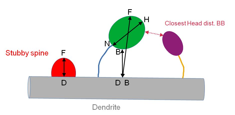
| 类型 | 要么是“有脖子的脊柱”,要么是“粗短的脊柱”。 “粗短脊柱”被定义为被分割的脊柱头部与树突直接接触的脊柱。注意,对于一些颈部粗的脊柱,分割过程可以使得整个脊柱被分割。然后颈部由一个体素组成。在这种情况下,脊柱被分类为“带颈部的脊柱”,但颈部长度=0。 |
| 头量(单位) | 脊柱头部的体积(微米立方) |
| 头部体积(像素) | 脊柱头部的体积(以体素为单位) |
| 颈长(单位) | 颈部长度(微米) |
| 颈长(像素) | 颈部长度(体素) |
| NtoH(单位) | 从颈部和头部接触点开始的最长脊柱头部直径(以微米为单位) |
| NtoH(像素) | 从颈部和头部之间的接触点开始的最长脊柱头部直径(以像素为单位) |
| 区。 BB(单位) | 树突模型和脊柱头部之间的边界到边界距离(以微米为单位) |
| 区。 BB(像素) | 树突模型和脊柱头部之间的边界到边界距离(以像素为单位) |
| 区。 DF(单位) | 最靠近树突头部的树突体素和距离树突最远的树突体素之间的微米距离(豪斯多夫距离) |
| 区。 DF(像素) | 最靠近树突头部的树突体素和距离树突最远的树突体素之间的像素距离(豪斯多夫距离) |
| 最近的头 BB | 基于边界到边界距离的最近脊柱头的标签 |
| 最近的头部距离BB | 脊椎头与最近的脊椎头之间的边界到边界距离 |
| 参数 | 描述 |
|---|---|
| 冲浪(单位) | 微米见方的脊柱头部表面 |
| 冲浪(像素) | 体素中脊柱头部的表面 |
| SurfCorr(像素) | 修正(平滑)体素表面。更多信息here |
| DCMin(像素) | 脊柱头部的最小直径(以像素为单位) |
| DCMax(像素) | 脊柱头部的最长直径(以像素为单位) |
| DC均值(像素) | 脊柱头部直径的平均值(以像素为单位) |
| DCMin(单位) | 脊柱头部的最小直径(以像素为单位) |
| DCMax(单位) | 脊柱头部的最长直径(以像素为单位) |
| DC 均值(单位) | 脊柱头部直径的平均值(以像素为单位) |
| 埃尔体积(单位) | 环绕脊柱头部的椭圆的体积,以微米立方为单位 |
| 埃尔斯帕内斯 | 椭圆体积与脊柱头部体积之比 |
| EllMajRadius(单位) | 椭圆长半径的长度(以微米为单位) |
| 埃隆 | 主半径长度与第二半径长度之比 |
| 平坦度 | 第二半径的长度与第三半径的长度之比。更多信息here |
| CX(像素)、CY(像素)、CZ(像素) | 脊柱头部的几何中心 |
| CMx(像素)、CMy(像素)、CMz(像素) | 脊柱头部的质心 |
| 比较(像素) | 紧凑性 |
| 球体(像素) | 球形度 |
| 比较 (像素) | 使用平滑表面计算的紧致度 |
| SpherCorr(像素) | 使用平滑表面计算的球形度。更多信息here |
| 最小 | 脊柱头部发现的最小强度值 |
| 最大 | 脊柱头部发现最大强度值 |
| 平均 | 脊柱头部的平均强度 |
| 标准差 | 脊柱头部强度值的标准偏差 |
| 积分密度 | 脊柱头部所有体素的强度值总和 |
| 模式 | 脊柱头部最常出现的强度值 |
| 费雷特(单位) | 脊柱头部的费雷特直径(微米) |
| 费雷特 (pxl) | 脊柱头部的 Feret 直径(以像素为单位) |
9.分析与其他对象的共定位或距离
您的图像堆栈可能不仅包含树突和棘,还可能包含另一个通道,例如轴突束、突触前或突触后蛋白质、小胶质细胞吞噬棘…… 您可能想要测量它们与分段脊柱头的共定位,或者测量脊柱头或颈部与感兴趣对象之间的最小 3D 距离。
SpotSpine 检索包含树突模型、脊柱头部、脊柱颈部通道的图像堆栈。分割复合材料并将分段的脊柱头部(或颈部或树突)保存为单通道图像堆栈。
分割其他感兴趣渠道的对象。
打开分段脊柱头/颈/树突的图像,并打开感兴趣的分段对象的图像。
运行插件 DiAna 以执行 3D 共定位或距离分析。 插件>DiAna>DiAna_Analyse DiAna 也可以进行批处理。
请记住,脊椎标记为 1、2、3…脊椎头部标记为 10、20、30…,其颈部标记为 15、25、35。因此,通过共定位分析获得的结果可以与通过 SpotSpine 获得的表中给出的测量结果相关联。
插件距离分析 - DiAna 的解释见 this page 和in the publication。
安装
-
下载以下 .jar 并将其复制到您的插件文件夹中 Spot_Spine.jar
- SNT和3D ImageJ Suite是可以通过更新站点安装的必需依赖项:
- 运行 Fiji Updater(Help,Help › Update…菜单中的倒数第二个条目)
- 单击管理更新站点
- 搜索 SNT 和 3D Image Suite 并选择各自的复选框
- 单击“应用更改”并重新启动斐济
- 提供图像堆栈和跟踪树突来测试插件。下载test image和SWC file of the dendrite
注意:
- 可以使用File › Show Folder › Plugins在文件系统中打开插件文件夹
- 3D 图像套件也可以是downloaded manually
引文
doi:10.12688/f1000research.146327.2
许可证
GPL 分发(参见第 license)。
更改日志
2025/01/29:v1.0.2 修正修改最大内核的错误 2024/08/30: v1.0.1 增强swc文件读取 2024/06/28:v1.0 调整树突形状和一些细节